Tutorial 9.1 - Linear mixed effects models
25 Apr 2018
Overview
For the purpose of reorientation and overall context, I present (again) the following representation of the linear model.

Of note, one of the primary assumptions of linear modelling is that the residuals are all independent of one another.
In the representation above, that is depicted by all the zeros in the covariance matrix.
If landscapes, individuals (subjects) etc were homogeneous, scientific experiments would be much easier to conduct. One of the greatest challenges in designing experiments (particular those in the field or those involving organisms) is to be able to minimize unexplained variability (noise) so as to maximize the likelihood of detecting any signals (effects). Alternatively, collecting additional covariates in an attempt to standardize or control for other influences is one of the common strategies used to attempt to reduce unexplained variability. However, this is a statistical method of attempting to control for predictable sources of noise.
When the source of heterogeneity is difficult to identify or measure, collecting additional covariates may not be effective. For example, in designing a field experiment that will involve measuring some property of a natural system (such as the abundance of a taxa within quadrats), we may be concerned that the underlying landscape varies enormously and that this variation could mask any treatment effects. That is, the unexplained variability will reduce the power to detect effects.
One way to compensate for this is to provision a very large number of replicates. However, this will necessarily require substantially more resources and effort. An alternative is to group together sets of sampling units at sufficiently small scales that the underlying conditions are relatively homogeneous. For example, rather than distribute the sampling units randomly (or haphazardly) throughout the landscape, clusters of sampling units (called blocks or plots) could be distributed throughout the landscape. Similarly, rather than subject each individual to a single treatment, each individual could be subjected to each of the treatments sequentially. In this way, the unexplained variability is based on variation within a cluster or individual - clusters and individuals partially act as their own control.
| Single factor | Nested |
|---|---|
 |
 |
Single factor | Randomized Complete Block |
 |
 |
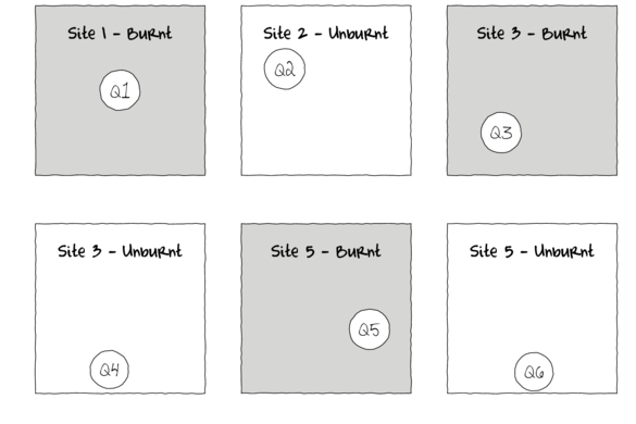
The series of figures above illustrate some of the issues addressed by hierarchical designs. The top left hand figure represents an example of a single factor design in which there are three sites (replicates) of the treatment factor (Burnt or Unburnt) and within each site there is a single haphazardly positioned quadrat from which some response was observed. If the conditions within a site a highly heterogeneous (perhaps the sites are not simple homogeneous patches of forest but rather are mixtures of forest types over undulating terrain), then obviously the locations of the quadrats within the landscapes are likely to be very influential. For example, if we were observing the abundance of ground dwelling spiders (as measured by the number of ground spiders captured in a single pit trap per site), yet each site had a mixture of habitats, ground cover and soil types, then the measured abundances of ground spiders is likely to be depended on exactly where within a site the pit trap is located.
Given this heterogeneity and considering there are only three replicates of each treatment, the amount of noise (unexplained variation) is likely to be very large and make it difficult to detect an effect of treatment. One solution would be to use more sites (perhaps many more sites) so that once averaged over a much larger set, the signal (treatment effect) starts to become apparent. However, this would require much more effort and resources and may not even be possible (may not be possible to obtain more burnt sites).
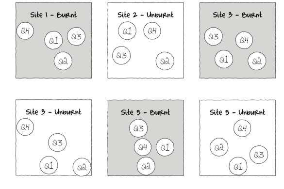
Another option is to use sub-replicates within each site. That is, rather than deploy a single pit trap, deploy many more. The top right figure shows the same Burnt and Unburnt sites, yet with four quadrats instead of one. If these subreplicates are positioned randomly throughout the heterogeneous landscape (thereby covering a range of conditions) and we average the observations across the subreplicates within each site, then hopefully we will have reduced the noise (unexplained variability).
Now lets focus on the bottom left figure above. This depicts a two factor (shape and color) design with each shape/color combination replicated four times. Importantly, note that unlike the previous nested example, in this example, the scale of the treatments is at the scale of the sampling unit. For example, in the Burnt/Unburnt example, a forest fire is at a much large scale that the typical sampling unit (a pit trap). However in the current example, the treatment (such as bait type, shaded/sheltered or not etc) can be applied at the scale of the sampling unit (pit trap, stream leaf pack etc). Again note that the quadrats (sampling units) are randomly positioned across the landscape. If again the landscape in which the quadrats are positioned is heterogeneous, the treatment effects could be masked or otherwise swamped by the extra variation due to location. For example, if the quadrats were placed in a stream (which we know are highly heterogeneous), the observed responses might be more influenced by where they are measured than any applied treatments.
In this case by grouping together each treatment combination into a smaller spatial scale (see lower right figure above) in which the conditions are likely to be more homogeneous, we should substantially reduce the amount of unexplained variation and thus increase the power to detect treatment effects. Importantly, to avoid introducing other systematic confounding effects, it is important that the treatments themselves be randomized within each group (block).
Such nested, blocking, repeated measures designs (collectively referred to as hierarchical designs as a result of sampling units being grouped within other 'larger scale' spatial or temporal units) are popular ways to reduce unexplained variability and thus increase power.
Obviously it is important that the groups of sampling units not be so close to one another that they directly influence one another. Nevertheless, sampling units within the groups (=blocks) are not strictly independent of one another. The unique underlying characteristics of the individual subject or block means that the multiple observations will likely be more similar to one another than they are to the observations collected from other subjects or blocks. Each subject or block will have their own unique baseline (e.g. heat rate) upon which the treatments act and it is the same baseline for all observations within the group.
This dependency issue can be tackled in much the same way as a lack of independence due to temporal or spatial autocorrelation (see Tutorial 8.3a). That is, by incorporating a variance structure that approximates the patterns of dependency. Indeed when fitting a hierarchical model, we are essentially fitting a model that incorporates a separate compound symmetry correlation structure for each group. Yet in order to leverage some other statistical information, rather than interact directly with the correlation structure, we typically engage a procedure that allows us to define the hierarchical structure of the data and the model will take care of the correlation structure for us.
Central to any discussion of hierarchical models in a frequentist paradigm is the notion of fixed and random factors or effects.
- Fixed factors - these are factors (continuous or categorical) whose measured levels you are specifically interested in. For example, we might have a treatment with levels 'high', 'medium' and 'low'. These are the only levels that we are interested in - we are not interested in extrapolating to other possible levels. Fixed effects are usually expressed as differences (or slopes).
- Random factors - these are factors (usually categorical) that represent groups sampling units (such as sites, subjects etc). We are typically not only interested in the effects of any one level of a random factor (such as how one individual compares to another), as the levels of random factors (the selected subjects or blocks) are assumed to be random representatives of a larger population. Instead, we are more interested in estimating how variable the different groups are to one another (how varied was the landscape or subjects). Note, the individual replicates are always considered random factors (since they are intended to be randomly selected representatives of which we are more interested in their collective variability than individual differences).
Hierarchical models contain a mixture of 'fixed' and 'random' effects and are therefore also referred to as Mixed Effects Models.
Recall that the typical linear model is of the form:
$$
\begin{align}
Y &\sim{} Normal(\mu, \sigma^2)\\
\mu &= \bf{X}\boldsymbol{\beta}
\end{align}
$$
where $\boldsymbol{\beta}$ represents the a vector of standard regression coefficients (such as intercept and slopes) being estimated and
$\bf{X}$ represents the predictor (model) matrix.
The typical mixed effects model is of the form:
$$
\begin{align}
Y &\sim{} Normal(\nu, \sigma^2)\\
\mu & = \bf{X}\boldsymbol{\beta} + \bf{Z}\boldsymbol{\gamma}\\
\boldsymbol{\gamma} &\sim{} MVNormal(0, \Sigma)\\
\Sigma &= f(\theta)
\end{align}
$$
where $\boldsymbol{\gamma}$ represents the a vector of coefficients associated with the random effects and
$\bf{Z}$ represents a matrix of the random terms.
Before proceeding any further, it might be a good idea to generate some data to assist us to visualize the concepts. We will generate a response (y) and continuous predictor (x) from 10 sampling units in each of 6 groups or blocks (block). A unit increase in x will be associated with a 1.5 times increase in y. The baseline of each block will be drawn from a normal distribution with a mean of 230 and a standard deviation of 20.
set.seed(1)
n.groups <- 6
n.sample <- 10
n <- n.groups * n.sample
block <- gl(n = n.groups, k = n.sample, lab = paste("Block",
    1:n.groups, sep = ""))
x <- runif(n, 0, 70)
mn <- mean(x)
sd <- sd(x)
cx <- (x - mn)  #/sd
Xmat <- model.matrix(~block * cx - 1 - cx)  #intercepts and slopes
Xmat <- model.matrix(~-1 + block + x)  #intercepts and slopes
intercept.mean <- 230
intercept.sd <- 20
slope.mean <- 1.5
# slope.sd <- 0.3
intercept.effects <- rnorm(n = n.groups, mean = intercept.mean,
    sd = intercept.sd)
# slope.effects <- rnorm(n=n.groups,
# mean=slope.mean, sd=slope.sd) #intercepts and
# slopes
slope.effects <- slope.mean
all.effects <- c(intercept.effects, slope.effects)
lin.pred <- Xmat[, ] %*% all.effects
eps <- rnorm(n = n, mean = 0, sd = 10)
y <- lin.pred + eps
data.hier <- data.frame(y = y, x = cx + mn, block = block)
head(data.hier)
         y        x  block
1 281.1091 18.58561 Block1
2 295.6535 26.04867 Block1
3 328.3234 40.09974 Block1
4 360.1672 63.57455 Block1
5 276.7050 14.11774 Block1
6 348.9709 62.88728 Block1
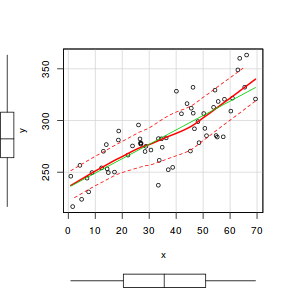
If we ignore the grouping dependency structure for a moment and proceed with simple linear regression (will will perform this via gls() so that we can directly compare it to models that incorporate correlation structures).
library(car)
scatterplot(y ~ x, data.hier)
library(nlme)
data.hier.gls <- gls(y ~ x, data.hier, method = "REML")
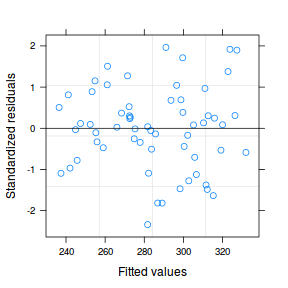
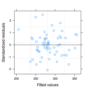
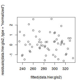
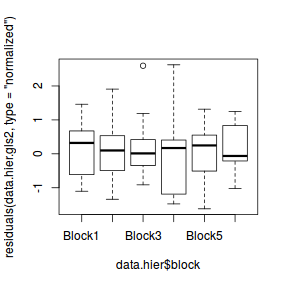
As always, we will explore the residuals. Firstly, we will explore the usual residual plot, then we will plot residuals against block. If there was no dependency structure (observations in groups were no more correlated to one another than they are to units in other groups), the spread of residuals should be similarly centered around zero for each block.
plot(data.hier.gls)
plot(residuals(data.hier.gls, type = "normalized") ~
    data.hier$block)
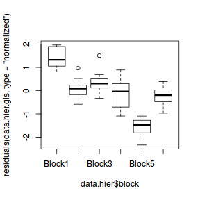
Detecting such issues in the residuals is perhaps not surprising, after all, this design is employed in situations where there are expected to be substantial differences between blocks. The model fitted above was not appropriate for two reasons.
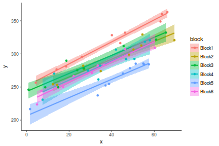
Firstly, it failed to account for the differences between different blocks and therefore the unexplained variation was inflated. We might be tempted to add the grouping variable (block) to the model in an attempt to account for some of this unexplained variability. In other words, could we not treat the analysis as a ANCOVA?
library(ggplot2)
ggplot(data.hier, aes(y = y, x = x, fill = block, color = block)) +
    geom_smooth(method = "lm") + geom_point() + theme_classic()
data.hier.gls1 <- gls(y ~ x + block, data.hier, method = "REML")
plot(data.hier.gls1)
plot(residuals(data.hier.gls1, type = "normalized") ~
    data.hier$block)
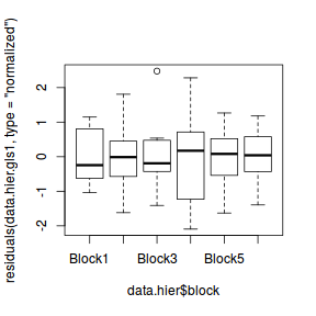
At first glance, this does seem to account for the different blocks. Although it is worth pointing out that to accounting for the block effects in this way has come at a substantial degrees of freedom cost. Since there are six blocks, we have invested an additional five degrees of freedom.
Unfortunately, (and secondly) this modelling option would also completely neglect the issue of dependency. Observations within blocks would not be considered independent.
A more appropriate alternative is to model in a correlation structure that accounts for the expected dependency. For a simple example such as this, we can construct the model that incorporates a separate compound symmetry correlation structure for each block. The somewhat peculiar 1|block notation in the corCompSymm() function indicates that the compound symmetry correlation structure should be allowed to differ for each block.
data.hier.gls2 <- gls(y ~ x, data.hier, correlation = corCompSymm(form = ~1 |
    block), method = "REML")
plot(residuals(data.hier.gls2, type = "normalized") ~
    fitted(data.hier.gls2))
plot(residuals(data.hier.gls2, type = "normalized") ~
    data.hier$block)
Whilst the above technique is adequate for enabling appropriate estimates and tests of the main effect of interest ( the relationship between y and x), it does not allow us to explore the breakdown of variance across the different hierarchical levels. It also makes it hard to impose additional correlation structures (such as those used to address temporal or spatial autocorrelation) on the data within each group.
So could we not just fit an ANCOVA along with the correlation structure?
data.hier.gls3 <- gls(y ~ x + block, data.hier, correlation = corCompSymm(form = ~1 |
    block), method = "REML")
There are two issues with this model. Firstly, a degree of freedom is lost for each estimate associated with the block factor. Since we are not specifically interested in the 'fixed' effects of a block (that is we are not interested in how each block differs from one of these blocks), generating such estimates only serves to rob the model of valuable degrees of freedom. Rather than estimate separate treatment effects for the levels of block, a more sensible approach would be to just estimate the added variance (a single parameter) due to the blocking effect (treat it as a 'random' effect).
Secondly, by incorporating block in the model as above, the intercept will represent the value of Y when X is zero for the first block. Again, we typically wish to generalize across all possible blocks. Thus it would be more sensible for the intercept to represent the value of Y when X is zero for the average block. Although we could construct this by altering the scale of the blocking factor and switching to something like sum contrasts, it turns out that there is a more natural solution.
Optimization
All parameter estimations require optimization. Optimization is a process in which a function is (typically) minimized over the range of parameter values. For many statistical modelling purposes, the function that we wish to optimize over (the objective function) is a likelihood function, and rather than minimize this function, we seek to maximize it. All optimization techniques are defined as minimizers and thus will be described as such. That said, maximizing a function is just the same as minimizing the negative of the function.
The basic idea is that assuming the model is correct and there is sufficient data, the likelihood of a function will be maximized near to the true values of the parameters. Moreover, the log-likelihood should be approximately quadratic in close proximity to the true values. Hence, here optimizing involves finding the values of the parameters that maximize a log-likelihood function. For simple models, this is relatively straight forward. Indeed for simple gaussian models, there is a closed form solution that can be solved by linear algebra. However, if the model is false or sample sizes are small or the function has local optima or plateaus, things become increasingly difficult.
Consider for a moment a direct search method of optimizing a single parameter function. You might start by applying a vector of possible parameter values and see which one yields the minimum (or maximum) log-likelihood. Obviously, the accuracy of this is going to depend on the granularity of the vector. If the vector only has five values, then unless you happen to be fortunate enough for the minimum to fall right on one of those values, then your estimates are not going to be all that accurate. On the other hand, if your vector is a sequence of one million values, then you are likely to get a very accurate estimate - although it will take substantially longer to get this estimate since you have to evaluate the function one million times instead of five. Furthermore, if the range of values represented by the vector is too narrow, there is a change that the true minimum lies outside this range. Hence, the accuracy of the optimization will depend on the appropriate choice of range and resolution, but that improvements in either will reduce speed.
If we take this approach a step further, we could start with a relatively wide and low resolution search grid and then iteratively 'zoom' in to yield progressively more accurate estimates. This approach of optimization is relatively simple, yet very slow and when there are more than a couple of parameters, the number of parameter combinations to evaluate will be a power function of the number of number of combinations. This will of course compound speed and resources issues. Hence for high dimensional likelihoods, more sophisticated solutions are required.
If on the other hand, we assume that the likelihood function is relatively smooth and has only a single minimum, we can leverage certain geometric properties in more sophisticated optimizations. For example, the derivative (gradient) of a function is equal to zero at the function's minimum. Similarly, for a multi-parameter likelihood function, partial derivatives (derivatives of each single parameter holding all other parameters constant) with respect to each of the parameters is a vector of zeros. Finding the roots (value associated with the derivative of zero), is still an iterative process. The search can be made more efficient by using the second order derivatives.
The Newton (or Newton-Ralphson) method iteratively estimates the partial parameter values as a linear extrapolation ($x_1 = x_0 - f(x_0)/f'(x_0)$) of the likelihood and derivative until it gets close enough to zero. When there are multiple parameters, this can be extended by linear extrapolation of the first and second order derivatives. This approach works reasonably well provided the initial parameter estimates are not wildly inaccurate and the functions themselves are differentiable. There are also alternatives that replace the derivatives and reciprocal of the second derivative with the inverse of the Hessian matrix. There are also further alternatives that use approximations of the Hessian that are built up from changes in the gradient over iterations.
Some approaches constrain the parameter estimates to certain bounding boxes (lower and upper bounds on each parameter) in order to restrict the search space, and thus speed up optimization. Consequently, there are a large number of optimizes available - each designed to address different difficult use cases. Rather than go through all of the optimizes, I will focus on just the general optimizers that are believed to good compromises between accuracy, speed and complexity.
- Nelder-Mead - is a direct search algorithm. Whilst it can be very slow, it is generally very reliable. Typically very slow when the number of parameters exceeds 10.
- BFGS - is a Quasi-Newton (Hessian-based) algorithm originally devised by Broyden, Fletcher, Goldfarb and Shanno in 1970
- L-BFGS-B - (Limited memory-BFGS-Box constraint) is a box constraint version of BFGS. It is most useful when the
- nlminb - is a more modern Quasi-Newton (Hessian-based) algorithm that accommodates box constraints. It is thought to be more robust than L-BFGS-B, particularly in more marginal cases where L-BFGS-B fails to converge.
- bobyqa - (Bound Optimization by Quadratic Approximation) is a quadratic approximation algorithm with support for box constraints that does not use derivatives.
There is no one best optimizer. An optimizer can fail for a number of reasons:
- iterations might reach a singular gradient and be forced to stop
- iterations exceed the maximum number of iterations without converging
- all variances must be positive
- covariance matrices must be positive definite
ML vs REML
Estimation for linear mixed effects models is via Maximum Likelihood (ML). That is, optimization finds the parameter values that maximize the (log) likelihood of the data. However, the ML method underestimates variance (random effects) parameters. The ML method yields biased estimates of random effects and unbiased estimates of fixed effects. Restricted Maximum Likelihood (REML) estimates of variance parameters are independent of the fixed effects estimates and therefore considered unbiased. In effect, they are the parameter values that minimize the (log) likelihood of the residuals. The REML method yields unbiased estimates of both fixed and random effects, yet are unsuitable for comparing fixed components across models.
- When comparing two models that differ only in their fixed structure, it is important that these models are fit using ML.
- When comparing two models that differ only in their random structure, it is important that these models are fit using REML.
- When exploring parameter estimates of a final model, the model should be fit using REML.
Linear mixed effects models in R
It is here that linear mixed effects models (LMM) models come in. In the following sections, I will introduce three packages for performing LMM. These are not the only packages, yet they do represent the major streams of routines. Briefly, these are:
- nlme package, originally writen for S, very widely used LMM implementation.
- lme4 package, the more modern (G)LMM implementation. Faster and handles crossed random effects but no 'R-side effects' (no autocorrelation or variance structures).
- glmmTMB package, an alternative LMM implementation.
Each of the above offer different underlying engines and capabilities and therefore choice of package, will dependend on the nature of the data and the desired model. Some of the major distinctions between these packages are summarised in the following table:
| nlme | lme4 | glmmTMB | |
|---|---|---|---|
| REML | Y | Y | N |
| optimizer | nlminb (default) or optim (BFGS or L-BFGS-B) | bobyqa (default) or Nelder_Mead | nlminb |
| spatial/temporal autocorrelation | Y | N | Y |
| variance structures | Y | N | Y |
| crossed random effects | N | Y | Y |
There are three main packages for LMM's in R that I intend to describe. Each have there own pros and cons and therefore, a working understanding of each implementation is still necessary.
data.hier.lme <- lme(y ~ x, random = ~1 | block, data.hier,
    method = "REML")
The hierarchical random effects structure is defined by the random= parameter. In this case, random=~1|block indicates that blocks are random effects and that the intercept should be allowed to vary per block. If we wished to allow the intercept and slope to vary for each block then the argument would have been something like random=~x|block. Note, that the constrained scatterplot above indicated that the slopes were similar for each group, so there was no real need for us to fit a random slope and intercepts model.
Nevertheless, we could explore whether there is a statistical basis to use the more complex model, by comparing the random intercept and random intercept/slope models via AIC.
data.hier.lme1 <- lme(y ~ x, random = ~x | block, data.hier, method = "REML")
Error in lme.formula(y ~ x, random = ~x | block, data.hier, method = "REML"): nlminb problem, convergence error code = 1
  message = iteration limit reached without convergence (10)
# Try the BFGS optimization algorithm instead
data.hier.lme1 <- lme(y ~ x, random = ~x | block, data.hier, method = "REML",
    control = lmeControl(opt = "optim", method = "BFGS"))
# compare the two models
anova(data.hier.lme, data.hier.lme1)
               Model df      AIC      BIC
data.hier.lme      1  4 458.9521 467.1938
data.hier.lme1     2  6 461.3996 473.7623
                  logLik   Test L.Ratio p-value
data.hier.lme  -225.4760
data.hier.lme1 -224.6998 1 vs 2 1.55245  0.4601
- actually, the more complex model using nlminb optimization failed to converge. That is, the iterative optimization process reached its maximum number of iterations and still failed to yield multiple outcomes that it considered similar enough to satisfy a convergence based stopping condition. The BFGS optimization seemed to have been successful..
- there is little support to indicate that the more complex random intercept/slope model is better than the simpler random intercept model
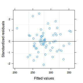
After fitting a model (any model), the model should always be validated to ensure that it is appropriate and has fit the data well. At the very least, this should involve an exploration of the residuals.
plot(data.hier.lme)
The fitted model is itself a list of class lme. Although it is possible to explore the contents of this list in order to extract the important components of perform additional analyses, it is usually more convenient to access the information via extractor functions and methods.
str(data.hier.lme)
List of 18
 $ modelStruct :List of 1
  ..$ reStruct:List of 1
  .. ..$ block:Classes 'pdLogChol', 'pdSymm', 'pdMat'  atomic [1:1] 0.71
  .. .. .. ..- attr(*, "formula")=Class 'formula'  language ~1
  .. .. .. .. .. ..- attr(*, ".Environment")=<environment: 0x74921e0>
  .. .. .. ..- attr(*, "Dimnames")=List of 2
  .. .. .. .. ..$ : chr "(Intercept)"
  .. .. .. .. ..$ : chr "(Intercept)"
  .. ..- attr(*, "settings")= num [1:4] 1 1 0 4
  .. ..- attr(*, "class")= chr "reStruct"
  .. ..- attr(*, "plen")= Named int 1
  .. .. ..- attr(*, "names")= chr "block"
  ..- attr(*, "settings")= num [1:4] 1 0 1 4
  ..- attr(*, "class")= chr [1:3] "lmeStructInt" "lmeStruct" "modelStruct"
  ..- attr(*, "pmap")= logi [1, 1] TRUE
  .. ..- attr(*, "dimnames")=List of 2
  .. .. ..$ : NULL
  .. .. ..$ : chr "reStruct"
  ..- attr(*, "fixedSigma")= logi FALSE
 $ dims        :List of 5
  ..$ N    : int 60
  ..$ Q    : int 1
  ..$ qvec : Named num [1:3] 1 0 0
  .. ..- attr(*, "names")= chr [1:3] "block" "" ""
  ..$ ngrps: Named int [1:3] 6 1 1
  .. ..- attr(*, "names")= chr [1:3] "block" "X" "y"
  ..$ ncol : Named num [1:3] 1 2 1
  .. ..- attr(*, "names")= chr [1:3] "block" "" ""
 $ contrasts   : Named list()
 $ coefficients:List of 2
  ..$ fixed : Named num [1:2] 232.82 1.46
  .. ..- attr(*, "names")= chr [1:2] "(Intercept)" "x"
  ..$ random:List of 1
  .. ..$ block: num [1:6, 1] 26.15 1.01 7.5 -1.87 -29.01 ...
  .. .. ..- attr(*, "dimnames")=List of 2
  .. .. .. ..$ : chr [1:6] "Block1" "Block2" "Block3" "Block4" ...
  .. .. .. ..$ : chr "(Intercept)"
 $ varFix      : num [1:2, 1:2] 61.20549 -0.14586 -0.14586 0.00407
  ..- attr(*, "dimnames")=List of 2
  .. ..$ : chr [1:2] "(Intercept)" "x"
  .. ..$ : chr [1:2] "(Intercept)" "x"
 $ sigma       : num 8.91
 $ apVar       : num [1:2, 1:2] 0.104932 -0.000227 -0.000227 0.009434
  ..- attr(*, "dimnames")=List of 2
  .. ..$ : chr [1:2] "reStruct.block" "lSigma"
  .. ..$ : chr [1:2] "reStruct.block" "lSigma"
  ..- attr(*, "Pars")= Named num [1:2] 2.9 2.19
  .. ..- attr(*, "names")= chr [1:2] "reStruct.block" "lSigma"
  ..- attr(*, "natural")= logi TRUE
 $ logLik      : num -225
 $ numIter     : NULL
 $ groups      :'data.frame':	60 obs. of  1 variable:
  ..$ block: Factor w/ 6 levels "Block1","Block2",..: 1 1 1 1 1 1 1 1 1 1 ...
 $ call        : language lme.formula(fixed = y ~ x, data = data.hier,      random = ~1 | block, method = "REML")
 $ terms       :Classes 'terms', 'formula'  language y ~ x
  .. ..- attr(*, "variables")= language list(y, x)
  .. ..- attr(*, "factors")= int [1:2, 1] 0 1
  .. .. ..- attr(*, "dimnames")=List of 2
  .. .. .. ..$ : chr [1:2] "y" "x"
  .. .. .. ..$ : chr "x"
  .. ..- attr(*, "term.labels")= chr "x"
  .. ..- attr(*, "order")= int 1
  .. ..- attr(*, "intercept")= int 1
  .. ..- attr(*, "response")= int 1
  .. ..- attr(*, ".Environment")=<environment: R_GlobalEnv>
  .. ..- attr(*, "predvars")= language list(y, x)
  .. ..- attr(*, "dataClasses")= Named chr [1:2] "numeric" "numeric"
  .. .. ..- attr(*, "names")= chr [1:2] "y" "x"
 $ method      : chr "REML"
 $ fitted      : num [1:60, 1:2] 260 271 291 326 253 ...
  ..- attr(*, "dimnames")=List of 2
  .. ..$ : chr [1:60] "1" "2" "3" "4" ...
  .. ..$ : chr [1:2] "fixed" "block"
 $ residuals   : num [1:60, 1:2] 21.2 24.8 37 34.6 23.3 ...
  ..- attr(*, "dimnames")=List of 2
  .. ..$ : chr [1:60] "1" "2" "3" "4" ...
  .. ..$ : chr [1:2] "fixed" "block"
  ..- attr(*, "std")= num [1:60] 8.91 8.91 8.91 8.91 8.91 ...
 $ fixDF       :List of 2
  ..$ X    : Named num [1:2] 53 53
  .. ..- attr(*, "names")= chr [1:2] "(Intercept)" "x"
  ..$ terms: Named num [1:2] 53 53
  .. ..- attr(*, "names")= chr [1:2] "(Intercept)" "x"
  ..- attr(*, "assign")=List of 2
  .. ..$ (Intercept): int 1
  .. ..$ x          : int 2
  ..- attr(*, "varFixFact")= num [1:2, 1:2] 7.4818 -2.2866 0 0.0638
 $ na.action   : NULL
 $ data        :'data.frame':	60 obs. of  3 variables:
  ..$ y    : num [1:60] 281 296 328 360 277 ...
  ..$ x    : num [1:60] 18.6 26 40.1 63.6 14.1 ...
  ..$ block: Factor w/ 6 levels "Block1","Block2",..: 1 1 1 1 1 1 1 1 1 1 ...
 - attr(*, "class")= chr "lme"
| Generic | Method | Package | Description |
|---|---|---|---|
| ACF | ACF.lme | nlme | Autocorrelation Function for lme Residuals |
| AIC | AIC | stats | Akaike's An Information Criterion |
| AICc | AICc | bbmle | Log likelihoods and model selection for mle2 objects |
| AICc | AICc | MuMIn | Second-order Akaike Information Criterion |
| allEffects | allEffects | effects | Functions For Constructing Effect Displays |
| allEffects | allEffects | RSiena | Internal data frame used to construct effect objects. |
| anova | anova.lme | nlme | Compare Likelihoods of Fitted Objects |
| augment | augment.lme | broom | Tidying methods for mixed effects models |
| coef | coef.lme | nlme | Extract lme Coefficients |
| Effect | Effect.lme | effects | Functions For Constructing Effect Displays for Many Modeling Paradigms |
| fitted | fitted.lme | nlme | Extract lme Fitted Values |
| fixef | fixef.lme | nlme | Extract Fixed Effects |
| glance | glance.lme | broom | Tidying methods for mixed effects models |
| glht | glht | lsmeans | 'lsmeans' support for 'glht' |
| glht | glht | multcomp | General Linear Hypotheses |
| intervals | intervals.lme | nlme | Confidence Intervals on lme Parameters |
| logLik | logLik.lme | nlme | Log-Likelihood of an lme Object |
| lsmeans | lsmeans | emmeans | Wrappers for alternative naming of EMMs |
| lsmeans | lsmeans | lmerTest | Calculates Least Squares Means and Confidence Intervals for the factors of a fixed part of mixed effects model of lmer object. |
| lsmeans | lsmeans | lsmeans | Least-squares means (or predicted marginal means) |
| plot | plot.lme | nlme | Plot an lme or nls object |
| predict | predict.lme | nlme | Predictions from an lme Object |
| ranef | ranef.lme | nlme | Extract lme Random Effects |
| residuals | residuals.lme | nlme | Extract lme Residuals |
| r.squaredGLMM | r.squaredGLMM.lme | MuMIn | Pseudo-R-squared for Generalized Mixed-Effect models |
| sigma | sigma.lme | nlme | Fitted lme Object |
| summary | summary.lme | nlme | Summarize an lme Object |
| tidy | tidy.lme | broom | Tidying methods for mixed effects models |
| vcov | vcov.lme | stats | Calculate Variance-Covariance Matrix for a Fitted Model Object |
methodsInfo = function(class = "lm") {
    require(tidyverse)
    meth = attr(methods(class = class), "info")
    .generic = meth$generic
    nms = rownames(meth)
    dat1 = list()
    for (i in seq_along(nms)) {
        a = help.search(paste0("^", nms[i], "$"), ignore.case = FALSE)
        aa = a$matches
        if (nrow(aa) == 0) {
            ## get the namespace of the full function
            nmspc = gsub("namespace:", "", getAnywhere(nms[i])$where[2])
            a = help.search(paste0("^", .generic[i],
                "$"), ignore.case = FALSE, field = "alias")
            aa = a$match %>% filter(Entry == .generic[i],
                Package == nmspc)
        }
        d = aa %>% dplyr::select(Title, Package, Entry,
            Field)
        d = d %>% distinct() %>% mutate(Generic = .generic[i]) %>%
            dplyr::select(Package, Generic, Entry,
                Title)
        dat1[[i]] = d
    }
    d = do.call("rbind", dat1)
    rownames(d) = NULL
    d %>% arrange(Package)
}
b = methodsInfo("lme")
b
   Package          Generic                Entry
1    broom          augment          augment.lme
2    broom           glance           glance.lme
3    broom             tidy             tidy.lme
4      car            Anova            Anova.lme
5      car      deltaMethod      deltaMethod.lme
6      car linearHypothesis linearHypothesis.lme
7      car       matchCoefs       matchCoefs.lme
8  effects           Effect           Effect.lme
9  lsmeans        lsm.basis            lsm.basis
10 lsmeans     recover.data         recover.data
11    MASS       extractAIC       extractAIC.lme
12    MASS            terms            terms.lme
13   MuMIn           coeffs               coeffs
14   MuMIn        coefTable        coefTable.lme
15   MuMIn      getAllTerms          getAllTerms
16   MuMIn    r.squaredGLMM        r.squaredGLMM
17    nlme              ACF              ACF.lme
18    nlme            anova            anova.lme
19    nlme          augPred          augPred.lme
20    nlme             coef             coef.lme
21    nlme      comparePred      comparePred.lme
22    nlme           fitted           fitted.lme
23    nlme            fixef                fixef
24    nlme          getData          getData.lme
25    nlme getGroupsFormula getGroupsFormula.lme
26    nlme        getGroups        getGroups.lme
27    nlme      getResponse          getResponse
28    nlme        getVarCov        getVarCov.lme
29    nlme        intervals        intervals.lme
30    nlme           logLik           logLik.lme
31    nlme            pairs            pairs.lme
32    nlme             plot             plot.lme
33    nlme          predict          predict.lme
34    nlme           qqnorm           qqnorm.lme
35    nlme            ranef            ranef.lme
36    nlme        residuals        residuals.lme
37    nlme            sigma            sigma.lme
38    nlme         simulate         simulate.lme
39    nlme          summary          summary.lme
40    nlme           update           update.lme
41    nlme          VarCorr          VarCorr.lme
42    nlme        Variogram        Variogram.lme
43   stats             vcov             vcov.lme
                                                                                      Title
1                                                  Tidying methods for mixed effects models
2                                                  Tidying methods for mixed effects models
3                                                  Tidying methods for mixed effects models
4                                               Anova Tables for Various Statistical Models
5  Estimate and Standard Error of a Nonlinear Function of Estimated Regression Coefficients
6                                                                    Test Linear Hypothesis
7                                                                    Test Linear Hypothesis
8                    Functions For Constructing Effect Displays for Many Modeling Paradigms
9                                           Support functions for creating a reference grid
10                                          Support functions for creating a reference grid
11                                            Choose a model by AIC in a Stepwise Algorithm
12                                            Choose a model by AIC in a Stepwise Algorithm
13                                                                  Model utility functions
14                                                                  Model utility functions
15                                                                  Model utility functions
16                                     Pseudo-R-squared for Generalized Mixed-Effect models
17                                               Autocorrelation Function for lme Residuals
18                                                    Compare Likelihoods of Fitted Objects
19                                                                    Augmented Predictions
20                                                                 Extract lme Coefficients
21                                                                      Compare Predictions
22                                                                Extract lme Fitted Values
23                                                                    Extract Fixed Effects
24                                                                  Extract lme Object Data
25                                                                 Extract Grouping Formula
26                                                                Extract lme Object Groups
27                                                 Extract Response Variable from an Object
28                                                       Extract variance-covariance matrix
29                                                   Confidence Intervals on lme Parameters
30                                                          Log-Likelihood of an lme Object
31                                                              Pairs Plot of an lme Object
32                                                                Plot an lme or nls object
33                                                           Predictions from an lme Object
34                            Normal Plot of Residuals or Random Effects from an lme Object
35                                                               Extract lme Random Effects
36                                                                    Extract lme Residuals
37                                                                        Fitted lme Object
38                                                       Simulate Results from 'lme' Models
39                                                                  Summarize an lme Object
40                                                              Linear Mixed-Effects Models
41                                              Extract variance and correlation components
42                                Calculate Semi-variogram for Residuals from an lme Object
43                           Calculate Variance-Covariance Matrix for a Fitted Model Object
For the sake of comparison, lets explore the output from the gls() and lme() routines.
# output of the gls with correlation structure for
# comparison
summary(data.hier.gls2)
Generalized least squares fit by REML
  Model: y ~ x
  Data: data.hier
       AIC      BIC   logLik
  458.9521 467.1938 -225.476

Correlation Structure: Compound symmetry
 Formula: ~1 | block
 Parameter estimate(s):
      Rho
0.8052553

Coefficients:
               Value Std.Error  t-value p-value
(Intercept) 232.8193  7.823394 29.75937       0
x             1.4591  0.063789 22.87392       0

 Correlation:
  (Intr)
x -0.292

Standardized residuals:
        Min          Q1         Med          Q3
-2.19174920 -0.59481155  0.05261311  0.59571239
        Max
 1.83321624

Residual standard error: 20.18017
Degrees of freedom: 60 total; 58 residual
# lme mixed effects model
summary(data.hier.lme)
Linear mixed-effects model fit by REML
 Data: data.hier
       AIC      BIC   logLik
  458.9521 467.1938 -225.476

Random effects:
 Formula: ~1 | block
        (Intercept) Residual
StdDev:    18.10888 8.905485

Fixed effects: y ~ x
               Value Std.Error DF  t-value
(Intercept) 232.8193  7.823393 53 29.75937
x             1.4591  0.063789 53 22.87392
            p-value
(Intercept)       0
x                 0
 Correlation:
  (Intr)
x -0.292

Standardized Within-Group Residuals:
        Min          Q1         Med          Q3
-2.09947262 -0.57994305 -0.04874031  0.56685096
        Max
 2.49464217

Number of Observations: 60
Number of Groups: 6
- the intercept represents the estimated value of y when x is equal to zero. As with regular regression, this is only really of some interest when the continuous predictor(s) are centered. Note that in the mixed effects context, this intercept represents the mean of the individual block intercepts (which we indicated could vary).
- the slope represents the common estimated rate of change in y per unit of change in x across all blocks (both observed and unobserved).
- the Correlation: the value of
-0.292275indicates that the approximate degree of correlation between the intercept and slope is-0.292275. Even the authors of the routine admit that the Correlation value is difficult to interpret, yet they suggest that it might sometimes speak to issues of multicollinearity when there are multiple predictors etc. or else that it might be difficult to interprete an effect of a predictor, if there is a high correlation between it and another estimate. - the lme summary includes estimates of the Random effects: These are the standard deviation of the individual block intercepts (between block variability) and the standard deviations of the observations around the individual block trends (within block effects, which in this case are the residuals). It is clear in this example, that there is more variability between blocks than within the blocks. Without the blocks, all the variability between the blocks would be unaccounted for and just considered residual unexplained noise. So the blocking has substantially reduced the unexplained variability and no doubt lead to more powerful fixed effects tests.
There are also a variety of other ways to summarize the linear mixed effects model. Below, I have included:
- an anova table that partitions sums of squares into explained and unexplain components - not very useful
- extract just the fixed effects coefficients
- extract just the random effects coefficients. Note, these are how much each indivual block intercept differs from the overal intercept and must sum to zero
- 95% confidence interval of the estimated parameters. These are very useful as they help when describing the magnitude of effects
- variance components expressed as proportion of total variability c.f. to standard deviation units displayed in regular summary output above.
anova(data.hier.lme, type = "marginal")
            numDF denDF  F-value p-value
(Intercept)     1    53 885.6203  <.0001
x               1    53 523.2164  <.0001
fixef(data.hier.lme)
(Intercept)           x
 232.819291    1.459101
ranef(data.hier.lme)
       (Intercept)
Block1   26.149932
Block2    1.013458
Block3    7.499362
Block4   -1.867983
Block5  -29.007062
Block6   -3.787707
intervals(data.hier.lme)
Approximate 95% confidence intervals

 Fixed effects:
                 lower       est.      upper
(Intercept) 217.127551 232.819291 248.511031
x             1.331156   1.459101   1.587045
attr(,"label")
[1] "Fixed effects:"

 Random Effects:
  Level: block
                   lower     est.    upper
sd((Intercept)) 9.597555 18.10888 34.16822

 Within-group standard error:
    lower      est.     upper
 7.361789  8.905485 10.772878
vc <- as.numeric(as.matrix(VarCorr(data.hier.lme))[,
    1])
vc/sum(vc)
[1] 0.8052553 0.1947447
Finally, there are also additional packages that offer simple and consistent output formats across a wide variety of tests.
library(broom)
tidy(data.hier.lme, effects = "fixed")
         term   estimate  std.error statistic
1 (Intercept) 232.819291 7.82339349  29.75937
2           x   1.459101 0.06378882  22.87392
       p.value
1 9.380593e-35
2 3.941855e-29
glance(data.hier.lme)
     sigma   logLik      AIC      BIC deviance
1 8.905485 -225.476 458.9521 467.1938       NA
library(lme4)
data.hier.lmer <- lmer(y ~ x + (1 | block), data = data.hier,
    REML = TRUE)
data.hier.lmer1 <- lmer(y ~ x + (x | block), data = data.hier,
    REML = TRUE)
AIC(data.hier.lmer, data.hier.lmer1)
                df      AIC
data.hier.lmer   4 458.9521
data.hier.lmer1  6 461.2017
anova(data.hier.lmer, data.hier.lmer1)
Data: data.hier
Models:
data.hier.lmer: y ~ x + (1 | block)
data.hier.lmer1: y ~ x + (x | block)
                Df    AIC    BIC  logLik deviance
data.hier.lmer   4 461.04 469.42 -226.52   453.04
data.hier.lmer1  6 463.22 475.79 -225.61   451.22
                 Chisq Chi Df Pr(>Chisq)
data.hier.lmer
data.hier.lmer1 1.8206      2     0.4024
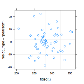
After fitting a model (any model), the model should always be validated to ensure that it is appropriate and has fit the data well. At the very least, this should involve an exploration of the residuals.
plot(data.hier.lmer)
The fitted model is itself a list of class lme. Although it is possible to explore the contents of this list in order to extract the important components of perform additional analyses, it is usually more convenient to access the information via extractor functions and methods.
str(data.hier.lmer)
Formal class 'lmerMod' [package "lme4"] with 13 slots
  ..@ resp   :Reference class 'lmerResp' [package "lme4"] with 9 fields
  .. ..$ Ptr    :<externalptr>
  .. ..$ mu     : num [1:60] 286 297 317 352 280 ...
  .. ..$ offset : num [1:60] 0 0 0 0 0 0 0 0 0 0 ...
  .. ..$ sqrtXwt: num [1:60] 1 1 1 1 1 1 1 1 1 1 ...
  .. ..$ sqrtrwt: num [1:60] 1 1 1 1 1 1 1 1 1 1 ...
  .. ..$ weights: num [1:60] 1 1 1 1 1 1 1 1 1 1 ...
  .. ..$ wtres  : num [1:60] -4.98 -1.32 10.84 8.44 -2.86 ...
  .. ..$ y      : num [1:60] 281 296 328 360 277 ...
  .. ..$ REML   : int 2
  .. ..and 28 methods, of which 14 are  possibly relevant:
  .. ..  allInfo, copy#envRefClass, initialize,
  .. ..  initialize#lmResp, initializePtr,
  .. ..  initializePtr#lmResp, objective, ptr,
  .. ..  ptr#lmResp, setOffset, setResp,
  .. ..  setWeights, updateMu, wrss
  ..@ Gp     : int [1:2] 0 6
  ..@ call   : language lmer(formula = y ~ x + (1 | block), data = data.hier,      REML = TRUE)
  ..@ frame  :'data.frame':	60 obs. of  3 variables:
  .. ..$ y    : num [1:60] 281 296 328 360 277 ...
  .. ..$ x    : num [1:60] 18.6 26 40.1 63.6 14.1 ...
  .. ..$ block: Factor w/ 6 levels "Block1","Block2",..: 1 1 1 1 1 1 1 1 1 1 ...
  .. ..- attr(*, "terms")=Classes 'terms', 'formula'  language y ~ x + (1 + block)
  .. .. .. ..- attr(*, "variables")= language list(y, x, block)
  .. .. .. ..- attr(*, "factors")= int [1:3, 1:2] 0 1 0 0 0 1
  .. .. .. .. ..- attr(*, "dimnames")=List of 2
  .. .. .. .. .. ..$ : chr [1:3] "y" "x" "block"
  .. .. .. .. .. ..$ : chr [1:2] "x" "block"
  .. .. .. ..- attr(*, "term.labels")= chr [1:2] "x" "block"
  .. .. .. ..- attr(*, "order")= int [1:2] 1 1
  .. .. .. ..- attr(*, "intercept")= int 1
  .. .. .. ..- attr(*, "response")= int 1
  .. .. .. ..- attr(*, ".Environment")=<environment: R_GlobalEnv>
  .. .. .. ..- attr(*, "predvars")= language list(y, x, block)
  .. .. .. ..- attr(*, "dataClasses")= Named chr [1:3] "numeric" "numeric" "factor"
  .. .. .. .. ..- attr(*, "names")= chr [1:3] "y" "x" "block"
  .. .. .. ..- attr(*, "predvars.fixed")= language list(y, x)
  .. .. .. ..- attr(*, "varnames.fixed")= chr [1:2] "y" "x"
  .. .. .. ..- attr(*, "predvars.random")= language list(y, block)
  .. ..- attr(*, "formula")=Class 'formula'  language y ~ x + (1 | block)
  .. .. .. ..- attr(*, ".Environment")=<environment: R_GlobalEnv>
  ..@ flist  :List of 1
  .. ..$ block: Factor w/ 6 levels "Block1","Block2",..: 1 1 1 1 1 1 1 1 1 1 ...
  .. ..- attr(*, "assign")= int 1
  ..@ cnms   :List of 1
  .. ..$ block: chr "(Intercept)"
  ..@ lower  : num 0
  ..@ theta  : num 2.03
  ..@ beta   : num [1:2] 232.82 1.46
  ..@ u      : num [1:6] 12.86 0.498 3.688 -0.919 -14.265 ...
  ..@ devcomp:List of 2
  .. ..$ cmp : Named num [1:10] 22.5 10.2 4212.8 387 4599.8 ...
  .. .. ..- attr(*, "names")= chr [1:10] "ldL2" "ldRX2" "wrss" "ussq" ...
  .. ..$ dims: Named int [1:12] 60 60 2 58 6 1 1 1 0 2 ...
  .. .. ..- attr(*, "names")= chr [1:12] "N" "n" "p" "nmp" ...
  ..@ pp     :Reference class 'merPredD' [package "lme4"] with 18 fields
  .. ..$ Lambdat:Formal class 'dgCMatrix' [package "Matrix"] with 6 slots
  .. .. .. ..@ i       : int [1:6] 0 1 2 3 4 5
  .. .. .. ..@ p       : int [1:7] 0 1 2 3 4 5 6
  .. .. .. ..@ Dim     : int [1:2] 6 6
  .. .. .. ..@ Dimnames:List of 2
  .. .. .. .. ..$ : NULL
  .. .. .. .. ..$ : NULL
  .. .. .. ..@ x       : num [1:6] 2.03 2.03 2.03 2.03 2.03 ...
  .. .. .. ..@ factors : list()
  .. ..$ LamtUt :Formal class 'dgCMatrix' [package "Matrix"] with 6 slots
  .. .. .. ..@ i       : int [1:60] 0 0 0 0 0 0 0 0 0 0 ...
  .. .. .. ..@ p       : int [1:61] 0 1 2 3 4 5 6 7 8 9 ...
  .. .. .. ..@ Dim     : int [1:2] 6 60
  .. .. .. ..@ Dimnames:List of 2
  .. .. .. .. ..$ : NULL
  .. .. .. .. ..$ : chr [1:60] "1" "2" "3" "4" ...
  .. .. .. ..@ x       : num [1:60] 2.03 2.03 2.03 2.03 2.03 ...
  .. .. .. ..@ factors : list()
  .. ..$ Lind   : int [1:6] 1 1 1 1 1 1
  .. ..$ Ptr    :<externalptr>
  .. ..$ RZX    : num [1:6, 1:2] 3.12 3.12 3.12 3.12 3.12 ...
  .. ..$ Ut     :Formal class 'dgCMatrix' [package "Matrix"] with 6 slots
  .. .. .. ..@ i       : int [1:60] 0 0 0 0 0 0 0 0 0 0 ...
  .. .. .. ..@ p       : int [1:61] 0 1 2 3 4 5 6 7 8 9 ...
  .. .. .. ..@ Dim     : int [1:2] 6 60
  .. .. .. ..@ Dimnames:List of 2
  .. .. .. .. ..$ : chr [1:6] "Block1" "Block2" "Block3" "Block4" ...
  .. .. .. .. ..$ : chr [1:60] "1" "2" "3" "4" ...
  .. .. .. ..@ x       : num [1:60] 1 1 1 1 1 1 1 1 1 1 ...
  .. .. .. ..@ factors : list()
  .. ..$ Utr    : num [1:6] 6424 5916 5759 5795 5386 ...
  .. ..$ V      : num [1:60, 1:2] 1 1 1 1 1 1 1 1 1 1 ...
  .. ..$ VtV    : num [1:2, 1:2] 60 0 2151 98116
  .. ..$ Vtr    : num [1:2] 17107 642529
  .. ..$ X      : num [1:60, 1:2] 1 1 1 1 1 1 1 1 1 1 ...
  .. .. ..- attr(*, "dimnames")=List of 2
  .. .. .. ..$ : chr [1:60] "1" "2" "3" "4" ...
  .. .. .. ..$ : chr [1:2] "(Intercept)" "x"
  .. .. ..- attr(*, "assign")= int [1:2] 0 1
  .. .. ..- attr(*, "msgScaleX")= chr(0)
  .. ..$ Xwts   : num [1:60] 1 1 1 1 1 1 1 1 1 1 ...
  .. ..$ Zt     :Formal class 'dgCMatrix' [package "Matrix"] with 6 slots
  .. .. .. ..@ i       : int [1:60] 0 0 0 0 0 0 0 0 0 0 ...
  .. .. .. ..@ p       : int [1:61] 0 1 2 3 4 5 6 7 8 9 ...
  .. .. .. ..@ Dim     : int [1:2] 6 60
  .. .. .. ..@ Dimnames:List of 2
  .. .. .. .. ..$ : chr [1:6] "Block1" "Block2" "Block3" "Block4" ...
  .. .. .. .. ..$ : chr [1:60] "1" "2" "3" "4" ...
  .. .. .. ..@ x       : num [1:60] 1 1 1 1 1 1 1 1 1 1 ...
  .. .. .. ..@ factors : list()
  .. ..$ beta0  : num [1:2] 0 0
  .. ..$ delb   : num [1:2] 232.82 1.46
  .. ..$ delu   : num [1:6] 12.86 0.498 3.688 -0.919 -14.265 ...
  .. ..$ theta  : num 2.03
  .. ..$ u0     : num [1:6] 0 0 0 0 0 0
  .. ..and 45 methods, of which 31 are  possibly relevant:
  .. ..  b, beta, CcNumer, copy#envRefClass,
  .. ..  initialize, initializePtr, installPars,
  .. ..  L, ldL2, ldRX2, linPred, P, ptr, RX,
  .. ..  RXdiag, RXi, setBeta0, setDelb, setDelu,
  .. ..  setTheta, setZt, solve, solveU, sqrL, u,
  .. ..  unsc, updateDecomp, updateL,
  .. ..  updateLamtUt, updateRes, updateXwts
  ..@ optinfo:List of 7
  .. ..$ optimizer: chr "bobyqa"
  .. ..$ control  :List of 1
  .. .. ..$ iprint: int 0
  .. ..$ derivs   :List of 2
  .. .. ..$ gradient: num 3.58e-08
  .. .. ..$ Hessian : num [1, 1] 4.21
  .. ..$ conv     :List of 2
  .. .. ..$ opt : int 0
  .. .. ..$ lme4: list()
  .. ..$ feval    : int 44
  .. ..$ warnings : list()
  .. ..$ val      : num 2.03
| Generic | Method | Package | Description |
|---|---|---|---|
| AIC | AIC | stats | Akaike's An Information Criterion |
| AICc | AICc | bbmle | Log likelihoods and model selection for mle2 objects |
| AICc | AICc | MuMIn | Second-order Akaike Information Criterion |
| allEffects | allEffects | effects | Functions For Constructing Effect Displays |
| allEffects | allEffects | RSiena | Internal data frame used to construct effect objects. |
| anova | anova.merMod | lme4 | Class "merMod" of Fitted Mixed-Effect Models |
| augment | augment.merMod | broom | Tidying methods for mixed effects models |
| coef | coef.merMod | lme4 | Class "merMod" of Fitted Mixed-Effect Models |
| confint | confint.merMod | lme4 | Compute Confidence Intervals for Parameters of a [ng]lmer Fit |
| Effect | Effect.merMod | effects | Functions For Constructing Effect Displays for Many Modeling Paradigms |
| fitted | fitted.merMod | lme4 | Class "merMod" of Fitted Mixed-Effect Models |
| fixef | fixef.merMod | lme4 | Extract fixed-effects estimates |
| glance | glance.merMod | broom | Tidying methods for mixed effects models |
| glht | glht | lsmeans | 'lsmeans' support for 'glht' |
| glht | glht | multcomp | General Linear Hypotheses |
| logLik | logLik.merMod | lme4 | Class "merMod" of Fitted Mixed-Effect Models |
| lsmeans | lsmeans | emmeans | Wrappers for alternative naming of EMMs |
| lsmeans | lsmeans | lmerTest | Calculates Least Squares Means and Confidence Intervals for the factors of a fixed part of mixed effects model of lmer object. |
| lsmeans | lsmeans | lsmeans | Least-squares means (or predicted marginal means) |
| plot | plot.merMod | lme4 | Diagnostic Plots for 'merMod' Fits |
| predict | predict.merMod | lme4 | Predictions from a model at new data values |
| ranef | ranef.merMod | lme4 | Extract the modes of the random effects |
| residuals | residuals.merMod | lme4 | residuals of merMod objects |
| r.squaredGLMM | r.squaredGLMM.merMod | MuMIn | Pseudo-R-squared for Generalized Mixed-Effect models |
| sigma | sigma.merMod | lme4 | Extract Residual Standard Deviation 'Sigma' |
| summary | summary.merMod | lme4 | Class "merMod" of Fitted Mixed-Effect Models |
| tidy | tidy.merMod | broom | Tidying methods for mixed effects models |
| vcov | vcov.merMod | lme4 | Class "merMod" of Fitted Mixed-Effect Models |
methodsInfo = function(class = "lm") {
    require(tidyverse)
    meth = attr(methods(class = class), "info")
    .generic = meth$generic
    nms = rownames(meth)
    dat1 = list()
    for (i in seq_along(nms)) {
        a = help.search(paste0("^", nms[i], "$"), ignore.case = FALSE)
        aa = a$matches
        if (nrow(aa) == 0) {
            ## get the namespace of the full function
            nmspc = gsub("namespace:", "", getAnywhere(nms[i])$where[2])
            a = help.search(paste0("^", .generic[i],
                "$"), ignore.case = FALSE, field = "alias")
            aa = a$match %>% filter(Entry == .generic[i],
                Package == nmspc)
        }
        d = aa %>% dplyr::select(Title, Package, Entry,
            Field)
        d = d %>% distinct() %>% mutate(Generic = .generic[i]) %>%
            dplyr::select(Package, Generic, Entry,
                Title)
        dat1[[i]] = d
    }
    d = do.call("rbind", dat1)
    rownames(d) = NULL
    d %>% arrange(Package)
}
b = methodsInfo("merMod")
b
   Package          Generic
1      arm       extractAIC
2    broom          augment
3    broom           glance
4    broom             tidy
5      car            Anova
6      car      deltaMethod
7      car linearHypothesis
8      car       matchCoefs
9  effects           Effect
10    lme4            anova
11    lme4      as.function
12    lme4             coef
13    lme4          confint
14    lme4         deviance
15    lme4      df.residual
16    lme4            drop1
17    lme4       extractAIC
18    lme4           family
19    lme4           fitted
20    lme4            fixef
21    lme4          formula
22    lme4          fortify
23    lme4             getL
24    lme4            getME
25    lme4        hatvalues
26    lme4           isGLMM
27    lme4            isLMM
28    lme4           isNLMM
29    lme4           isREML
30    lme4           logLik
31    lme4      model.frame
32    lme4     model.matrix
33    lme4            ngrps
34    lme4             nobs
35    lme4             plot
36    lme4          predict
37    lme4            print
38    lme4          profile
39    lme4            ranef
40    lme4            refit
41    lme4          refitML
42    lme4        residuals
43    lme4             show
44    lme4            sigma
45    lme4         simulate
46    lme4          summary
47    lme4            terms
48    lme4           update
49    lme4          VarCorr
50    lme4             vcov
51    lme4          weights
52 lsmeans        lsm.basis
53 lsmeans     recover.data
54   MuMIn           coeffs
55   MuMIn    r.squaredGLMM
                     Entry
1        extractAIC.merMod
2           augment.merMod
3            glance.merMod
4              tidy.merMod
5             Anova.merMod
6       deltaMethod.merMod
7  linearHypothesis.merMod
8        matchCoefs.merMod
9            Effect.merMod
10            anova.merMod
11      as.function.merMod
12             coef.merMod
13          confint.merMod
14         deviance.merMod
15      df.residual.merMod
16            drop1.merMod
17       extractAIC.merMod
18           family.merMod
19           fitted.merMod
20            fixef.merMod
21          formula.merMod
22          fortify.merMod
23      getL,merMod-method
24            getME.merMod
25        hatvalues.merMod
26           isGLMM.merMod
27            isLMM.merMod
28           isNLMM.merMod
29           isREML.merMod
30           logLik.merMod
31      model.frame.merMod
32     model.matrix.merMod
33            ngrps.merMod
34             nobs.merMod
35             plot.merMod
36          predict.merMod
37            print.merMod
38          profile.merMod
39            ranef.merMod
40            refit.merMod
41          refitML.merMod
42        residuals.merMod
43      show,merMod-method
44            sigma.merMod
45         simulate.merMod
46          summary.merMod
47            terms.merMod
48           update.merMod
49          VarCorr.merMod
50             vcov.merMod
51          weights.merMod
52               lsm.basis
53            recover.data
54                  coeffs
55           r.squaredGLMM
                                                                                      Title
1                                                    Extract AIC and DIC from a 'mer' model
2                                                  Tidying methods for mixed effects models
3                                                  Tidying methods for mixed effects models
4                                                  Tidying methods for mixed effects models
5                                               Anova Tables for Various Statistical Models
6  Estimate and Standard Error of a Nonlinear Function of Estimated Regression Coefficients
7                                                                    Test Linear Hypothesis
8                                                                    Test Linear Hypothesis
9                    Functions For Constructing Effect Displays for Many Modeling Paradigms
10                                             Class "merMod" of Fitted Mixed-Effect Models
11                                             Class "merMod" of Fitted Mixed-Effect Models
12                                             Class "merMod" of Fitted Mixed-Effect Models
13                            Compute Confidence Intervals for Parameters of a [ng]lmer Fit
14                                             Class "merMod" of Fitted Mixed-Effect Models
15                                             Class "merMod" of Fitted Mixed-Effect Models
16                    Drop all possible single fixed-effect terms from a mixed effect model
17                                             Class "merMod" of Fitted Mixed-Effect Models
18                                             Class "merMod" of Fitted Mixed-Effect Models
19                                             Class "merMod" of Fitted Mixed-Effect Models
20                                                          Extract fixed-effects estimates
21                                             Class "merMod" of Fitted Mixed-Effect Models
22                                          add information to data based on a fitted model
23                  Extract or Get Generalized Components from a Fitted Mixed Effects Model
24                  Extract or Get Generalized Components from a Fitted Mixed Effects Model
25                                                      Diagonal elements of the hat matrix
26                                                          Check characteristics of models
27                                                          Check characteristics of models
28                                                          Check characteristics of models
29                                                          Check characteristics of models
30                                             Class "merMod" of Fitted Mixed-Effect Models
31                                             Class "merMod" of Fitted Mixed-Effect Models
32                                             Class "merMod" of Fitted Mixed-Effect Models
33                                             Class "merMod" of Fitted Mixed-Effect Models
34                                             Class "merMod" of Fitted Mixed-Effect Models
35                                                       Diagnostic Plots for 'merMod' Fits
36                                              Predictions from a model at new data values
37                                             Class "merMod" of Fitted Mixed-Effect Models
38                                                        Profile method for merMod objects
39                                                  Extract the modes of the random effects
40                                         Refit a (merMod) Model with a Different Response
41                                            Refit a Model by Maximum Likelihood Criterion
42                                                              residuals of merMod objects
43                                             Class "merMod" of Fitted Mixed-Effect Models
44                                              Extract Residual Standard Deviation 'Sigma'
45                                                  Simulate Responses From 'merMod' Object
46                                             Class "merMod" of Fitted Mixed-Effect Models
47                                             Class "merMod" of Fitted Mixed-Effect Models
48                                             Class "merMod" of Fitted Mixed-Effect Models
49                                              Extract Variance and Correlation Components
50                                             Class "merMod" of Fitted Mixed-Effect Models
51                                             Class "merMod" of Fitted Mixed-Effect Models
52                                          Support functions for creating a reference grid
53                                          Support functions for creating a reference grid
54                                                                  Model utility functions
55                                     Pseudo-R-squared for Generalized Mixed-Effect models
summary(data.hier.lmer)
Linear mixed model fit by REML ['lmerMod']
Formula: y ~ x + (1 | block)
   Data: data.hier

REML criterion at convergence: 451

Scaled residuals:
     Min       1Q   Median       3Q      Max
-2.09947 -0.57994 -0.04874  0.56685  2.49464

Random effects:
 Groups   Name        Variance Std.Dev.
 block    (Intercept) 327.93   18.109
 Residual              79.31    8.905
Number of obs: 60, groups:  block, 6

Fixed effects:
             Estimate Std. Error t value
(Intercept) 232.81929    7.82339   29.76
x             1.45910    0.06379   22.87

Correlation of Fixed Effects:
  (Intr)
x -0.292
Conclusions - we see that although each routine yeilds a slightly different output, the estimations are identical.
- the intercept represents the estimated value of y when x is equal to zero. As with regular regression, this is only really of some interest when the continuous predictor(s) are centered. Note that in the mixed effects context, this intercept represents the mean of the individual block intercepts (which we indicated could vary).
- the slope represents the common estimated rate of change in y per unit of change in x across all blocks (both observed and unobserved).
- the Correlation: the value of
-0.292275indicates that the approximate degree of correlation between the intercept and slope is-0.292275. Even the authors of the routine admit that the Correlation value is difficult to interpret, yet they suggest that it might sometimes speak to issues of multicollinearity when there are multiple predictors etc. or else that it might be difficult to interprete an effect of a predictor, if there is a high correlation between it and another estimate. - the lmer summary includes estimates of the Random effects: These are provided in units of both standard deviation and variance of the individual block intercepts (between block variability) and the standard deviations (and variance) of the observations around the individual block trends (within block effects, which in this case are the residuals). It is clear in this example, that there is more variability between blocks than within the blocks. Without the blocks, all the variability between the blocks would be unaccounted for and just considered residual unexplained noise. So the blocking has substantially reduced the unexplained variability and no doubt lead to more powerful fixed effects tests.
There are also a variety of other ways to summarize the linear mixed effects model. Below, I have included:
- an anova table that partitions sums of squares into explained and unexplain components - not very useful
- extract just the fixed effects coefficients
- extract just the random effects coefficients. Note, these are how much each indivual block intercept differs from the overal intercept and must sum to zero
- 95% confidence interval of the estimated parameters. These are very useful as they help when describing the magnitude of effects
- variance components expressed as proportion of total variability c.f. to standard deviation units displayed in regular summary output above.
anova(data.hier.lmer, type = "marginal")
Analysis of Variance Table
  Df Sum Sq Mean Sq F value
x  1  41495   41495  523.22
fixef(data.hier.lmer)
(Intercept)           x
 232.819291    1.459101
ranef(data.hier.lmer)
$block
       (Intercept)
Block1   26.149932
Block2    1.013458
Block3    7.499362
Block4   -1.867983
Block5  -29.007062
Block6   -3.787707
confint(data.hier.lmer)
                 2.5 %     97.5 %
.sig01       10.000903  33.426060
.sigma        7.388234  10.789617
(Intercept) 216.495897 249.098759
x             1.332559   1.584745
vc <- as.data.frame(VarCorr(data.hier.lmer))[, "vcov"]
vc/sum(vc)
[1] 0.8052553 0.1947447
Finally, there are also additional packages that offer simple and consistent output formats across a wide variety of tests.
library(broom)
tidy(data.hier.lmer, effects = "fixed")
         term   estimate  std.error statistic
1 (Intercept) 232.819291 7.82339353  29.75937
2           x   1.459101 0.06378882  22.87392
glance(data.hier.lmer)
     sigma   logLik      AIC      BIC deviance
1 8.905485 -225.476 458.9521 467.3294 453.1143
  df.residual
1          56
You might have noticed an absence of p-values from the output above. This is not a mistake, it is deliberate. The lme4 package authors maintain that their is sufficient debate and disagreement over how to calculate degrees of freedom in the present of random effects, that they have elected not to provide residual degrees of freedom and therefore p-values.
As a pragmatic alternative, there is another package (lmerTest) that temporarily replaces the lmer() function as defined in lme4 with one of its own. Its version, has a numberof popular ways of estimating residual degrees of freedom and thus p-values. To take affect, the model must be run after the package is loaded.
library(lmerTest)
data.lmer = update(data.hier.lmer)
summary(data.hier.lmer)
Linear mixed model fit by REML ['lmerMod']
Formula: y ~ x + (1 | block)
   Data: data.hier

REML criterion at convergence: 451

Scaled residuals:
     Min       1Q   Median       3Q      Max
-2.09947 -0.57994 -0.04874  0.56685  2.49464

Random effects:
 Groups   Name        Variance Std.Dev.
 block    (Intercept) 327.93   18.109
 Residual              79.31    8.905
Number of obs: 60, groups:  block, 6

Fixed effects:
             Estimate Std. Error t value
(Intercept) 232.81929    7.82339   29.76
x             1.45910    0.06379   22.87

Correlation of Fixed Effects:
  (Intr)
x -0.292
Mixed effects models can also be fit using the Template Model Builder automatic differentiation engine via the glmmTMB() function from a package with the same name. glmmTMB() is able to fit similar models to lmer(), yet can also incorporate more complex features such as zero inflation and temporal autocorrelation. Random effects are assumed to be Gaussian on the scale of the linear predictor and are integrated out via Laplace approximation. On the downsides, REML is not available for this technique yet and nor is Gauss-Hermite quadrature (which can be useful when dealing with small sample sizes and non-gaussian errors).
Importantly, glmmTMB prefers that for more complex models (multiple predictors or random intercept/slopes), the continuous predictors are first scaled. When scaling data, make sure you remember that you have scaled the data when interpreting the results.
data.hier = data.hier %>% mutate(cx = as.vector(scale(x)))
library(glmmTMB)
data.hier.glmmTMB <- glmmTMB(y ~ x + (1 | block), data = data.hier)
data.hier.glmmTMB1 <- glmmTMB(y ~ cx + (cx | block),
    data = data.hier)
AIC(data.hier.glmmTMB, data.hier.glmmTMB1)
                   df      AIC
data.hier.glmmTMB   4 461.0447
data.hier.glmmTMB1  6 463.2242
anova(data.hier.glmmTMB, data.hier.glmmTMB1)
Data: data.hier
Models:
data.hier.glmmTMB: y ~ x + (1 | block), zi=~0, disp=~1
data.hier.glmmTMB1: y ~ cx + (cx | block), zi=~0, disp=~1
                   Df    AIC    BIC  logLik
data.hier.glmmTMB   4 461.04 469.42 -226.52
data.hier.glmmTMB1  6 463.22 475.79 -225.61
                   deviance  Chisq Chi Df
data.hier.glmmTMB    453.04
data.hier.glmmTMB1   451.22 1.8206      2
                   Pr(>Chisq)
data.hier.glmmTMB
data.hier.glmmTMB1     0.4024
After fitting a model (any model), the model should always be validated to ensure that it is appropriate and has fit the data well. At the very least, this should involve an exploration of the residuals.
ggplot(data = NULL) + geom_point(aes(y = residuals(data.hier.glmmTMB,
    type = "pearson", scaled = TRUE), x = fitted(data.hier.glmmTMB)))
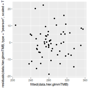
The fitted model is itself a list of class lme. Although it is possible to explore the contents of this list in order to extract the important components of perform additional analyses, it is usually more convenient to access the information via extractor functions and methods.
str(data.hier.glmmTMB)
List of 7
 $ obj      :List of 10
  ..$ par     : Named num [1:4] 1 1 0 0
  .. ..- attr(*, "names")= chr [1:4] "beta" "beta" "betad" "theta"
  ..$ fn      :function (x = last.par[-random], ...)
  ..$ gr      :function (x = last.par[-random], ...)
  ..$ he      :function (x = last.par[-random], ...)
  ..$ hessian : logi FALSE
  ..$ method  : chr "BFGS"
  ..$ retape  :function ()
  ..$ env     :<environment: 0x9824038>
  ..$ report  :function (par = last.par)
  ..$ simulate:function (par = last.par, complete = FALSE)
 $ fit      :List of 7
  ..$ par        : Named num [1:4] 232.83 1.46 4.35 2.8
  .. ..- attr(*, "names")= chr [1:4] "beta" "beta" "betad" "theta"
  ..$ objective  : num 227
  ..$ convergence: int 0
  ..$ iterations : int 41
  ..$ evaluations: Named int [1:2] 46 42
  .. ..- attr(*, "names")= chr [1:2] "function" "gradient"
  ..$ message    : chr "relative convergence (4)"
  ..$ parfull    : Named num [1:10] 232.83 1.46 26.04 1.01 7.47 ...
  .. ..- attr(*, "names")= chr [1:10] "beta" "beta" "b" "b" ...
 $ sdr      :List of 10
  ..$ value          : num(0)
  ..$ sd             : num(0)
  ..$ cov            : logi[0 , 0 ]
  ..$ par.fixed      : Named num [1:4] 232.83 1.46 4.35 2.8
  .. ..- attr(*, "names")= chr [1:4] "beta" "beta" "betad" "theta"
  ..$ cov.fixed      : num [1:4, 1:4] 51.75932 -0.14317 0.00266 -0.01236 -0.14317 ...
  .. ..- attr(*, "dimnames")=List of 2
  .. .. ..$ : chr [1:4] "beta" "beta" "betad" "theta"
  .. .. ..$ : chr [1:4] "beta" "beta" "betad" "theta"
  ..$ pdHess         : logi TRUE
  ..$ gradient.fixed : num [1:4] -2.73e-07 2.70e-05 4.72e-05 -2.15e-05
  ..$ par.random     : Named num [1:6] 26.04 1.01 7.47 -1.86 -28.88 ...
  .. ..- attr(*, "names")= chr [1:6] "b" "b" "b" "b" ...
  ..$ diag.cov.random: num [1:6] 51.9 51.7 51.8 51.6 52.1 ...
  ..$ env            :<environment: 0x97423b8>
  ..- attr(*, "class")= chr "sdreport"
 $ call     : language glmmTMB(formula = y ~ x + (1 | block), data = data.hier,      ziformula = ~0, dispformula = ~1)
 $ frame    :'data.frame':	60 obs. of  3 variables:
  ..$ y    : num [1:60] 281 296 328 360 277 ...
  ..$ x    : num [1:60] 18.6 26 40.1 63.6 14.1 ...
  ..$ block: Factor w/ 6 levels "Block1","Block2",..: 1 1 1 1 1 1 1 1 1 1 ...
  ..- attr(*, "terms")=Classes 'terms', 'formula'  language y ~ x + (1 + block) + 0 + 1
  .. .. ..- attr(*, "variables")= language list(y, x, block)
  .. .. ..- attr(*, "factors")= int [1:3, 1:2] 0 1 0 0 0 1
  .. .. .. ..- attr(*, "dimnames")=List of 2
  .. .. .. .. ..$ : chr [1:3] "y" "x" "block"
  .. .. .. .. ..$ : chr [1:2] "x" "block"
  .. .. ..- attr(*, "term.labels")= chr [1:2] "x" "block"
  .. .. ..- attr(*, "order")= int [1:2] 1 1
  .. .. ..- attr(*, "intercept")= int 1
  .. .. ..- attr(*, "response")= int 1
  .. .. ..- attr(*, ".Environment")=<environment: R_GlobalEnv>
  .. .. ..- attr(*, "predvars")= language list(y, x, block)
  .. .. ..- attr(*, "dataClasses")= Named chr [1:3] "numeric" "numeric" "factor"
  .. .. .. ..- attr(*, "names")= chr [1:3] "y" "x" "block"
 $ modelInfo:List of 7
  ..$ nobs   : int 60
  ..$ respCol: Named int 1
  .. ..- attr(*, "names")= chr "y"
  ..$ grpVar : chr "block"
  ..$ family :List of 11
  .. ..$ family    : chr "gaussian"
  .. ..$ link      : chr "identity"
  .. ..$ linkfun   :function (mu)
  .. ..$ linkinv   :function (eta)
  .. ..$ variance  :function (mu)
  .. ..$ dev.resids:function (y, mu, wt)
  .. ..$ aic       :function (y, n, mu, wt, dev)
  .. ..$ mu.eta    :function (eta)
  .. ..$ initialize:  expression({     n <- rep.int(1, nobs)     if (is.null(etastart) && is.null(start) &&          is.null(mustart) && ((family$link ==          "inverse" && any(y == 0)) || (family$link ==          "log" && any(y <= 0))))          stop("cannot find valid starting values: please specify some")     mustart <- y })
  .. ..$ validmu   :function (mu)
  .. ..$ valideta  :function (eta)
  .. ..- attr(*, "class")= chr "family"
  ..$ reTrms :List of 2
  .. ..$ cond:List of 3
  .. .. ..$ cnms :List of 1
  .. .. .. ..$ block: chr "(Intercept)"
  .. .. ..$ flist:List of 1
  .. .. .. ..$ block: Factor w/ 6 levels "Block1","Block2",..: 1 1 1 1 1 1 1 1 1 1 ...
  .. .. .. ..- attr(*, "assign")= int 1
  .. .. ..$ terms:List of 1
  .. .. .. ..$ fixed:Classes 'terms', 'formula'  language y ~ x
  .. .. .. .. .. ..- attr(*, "variables")= language list(y, x)
  .. .. .. .. .. ..- attr(*, "factors")= int [1:2, 1] 0 1
  .. .. .. .. .. .. ..- attr(*, "dimnames")=List of 2
  .. .. .. .. .. .. .. ..$ : chr [1:2] "y" "x"
  .. .. .. .. .. .. .. ..$ : chr "x"
  .. .. .. .. .. ..- attr(*, "term.labels")= chr "x"
  .. .. .. .. .. ..- attr(*, "order")= int 1
  .. .. .. .. .. ..- attr(*, "intercept")= int 1
  .. .. .. .. .. ..- attr(*, "response")= int 1
  .. .. .. .. .. ..- attr(*, ".Environment")=<environment: R_GlobalEnv>
  .. .. .. .. .. ..- attr(*, "predvars")= language list(y, x)
  .. .. .. .. .. ..- attr(*, "dataClasses")= Named chr [1:2] "numeric" "numeric"
  .. .. .. .. .. .. ..- attr(*, "names")= chr [1:2] "y" "x"
  .. ..$ zi  :List of 1
  .. .. ..$ terms:List of 1
  .. .. .. ..$ fixed:Classes 'terms', 'formula'  language ~0
  .. .. .. .. .. ..- attr(*, "variables")= language list()
  .. .. .. .. .. ..- attr(*, "factors")= int(0)
  .. .. .. .. .. ..- attr(*, "term.labels")= chr(0)
  .. .. .. .. .. ..- attr(*, "order")= int(0)
  .. .. .. .. .. ..- attr(*, "intercept")= int 0
  .. .. .. .. .. ..- attr(*, "response")= int 0
  .. .. .. .. .. ..- attr(*, ".Environment")=<environment: R_GlobalEnv>
  .. .. .. .. .. ..- attr(*, "predvars")= language list()
  .. .. .. .. .. ..- attr(*, "dataClasses")= Named chr(0)
  .. .. .. .. .. .. ..- attr(*, "names")= chr(0)
  ..$ reStruc:List of 2
  .. ..$ condReStruc:List of 1
  .. .. ..$ 1 | block:List of 4
  .. .. .. ..$ blockReps    : num 6
  .. .. .. ..$ blockSize    : num 1
  .. .. .. ..$ blockNumTheta: num 1
  .. .. .. ..$ blockCode    : Named num 1
  .. .. .. .. ..- attr(*, "names")= chr "us"
  .. ..$ ziReStruc  : list()
  ..$ allForm:List of 4
  .. ..$ combForm   :Class 'formula'  language y ~ x + (1 + block) + 0 + 1
  .. .. .. ..- attr(*, ".Environment")=<environment: R_GlobalEnv>
  .. ..$ formula    :Class 'formula'  language y ~ x + (1 | block)
  .. .. .. ..- attr(*, ".Environment")=<environment: R_GlobalEnv>
  .. ..$ ziformula  :Class 'formula'  language ~0
  .. .. .. ..- attr(*, ".Environment")=<environment: R_GlobalEnv>
  .. ..$ dispformula:Class 'formula'  language ~1
  .. .. .. ..- attr(*, ".Environment")=<environment: R_GlobalEnv>
 $ fitted   : NULL
 - attr(*, "class")= chr "glmmTMB"
| Generic | Method | Package | Description |
|---|---|---|---|
| AIC | AIC | stats | Akaike's An Information Criterion |
| confint | confint.glmmTMB | glmmTMB | Calculate confidence intervals |
| fixef | fixef.glmmTMB | glmmTMB | Extract fixed-effects estimates |
| predict | predict.glmmTMB | glmmTMB | prediction |
| ranef | ranef.glmmTMB | glmmTMB | Extract Random Effects |
| residuals | residuals.glmmTMB | glmmTMB | Compute residuals for a glmmTMB object |
| sigma | sigma.glmmTMB | glmmTMB | Extract residual standard deviation or dispersion parameter |
| vcov | vcov.glmmTMB | glmmTMB | Calculate Variance-Covariance Matrix for a Fitted glmmTMB model |
methodsInfo = function(class = "lm") {
    require(tidyverse)
    meth = attr(methods(class = class), "info")
    .generic = meth$generic
    nms = rownames(meth)
    dat1 = list()
    for (i in seq_along(nms)) {
        a = help.search(paste0("^", nms[i], "$"), ignore.case = FALSE)
        aa = a$matches
        if (nrow(aa) == 0) {
            ## get the namespace of the full function
            nmspc = gsub("namespace:", "", getAnywhere(nms[i])$where[2])
            a = help.search(paste0("^", .generic[i],
                "$"), ignore.case = FALSE, field = "alias")
            aa = a$match %>% filter(Entry == .generic[i],
                Package == nmspc)
        }
        d = aa %>% dplyr::select(Title, Package, Entry,
            Field)
        d = d %>% distinct() %>% mutate(Generic = .generic[i]) %>%
            dplyr::select(Package, Generic, Entry,
                Title)
        dat1[[i]] = d
    }
    d = do.call("rbind", dat1)
    rownames(d) = NULL
    d %>% arrange(Package)
}
b = methodsInfo("glmmTMB")
b
   Package   Generic             Entry
1  glmmTMB   confint   confint.glmmTMB
2  glmmTMB    family    family_glmmTMB
3  glmmTMB     fixef     fixef.glmmTMB
4  glmmTMB     getME     getME.glmmTMB
5  glmmTMB   predict   predict.glmmTMB
6  glmmTMB   profile   profile.glmmTMB
7  glmmTMB     ranef     ranef.glmmTMB
8  glmmTMB residuals residuals.glmmTMB
9  glmmTMB     sigma     sigma.glmmTMB
10 glmmTMB  simulate  simulate.glmmTMB
11 glmmTMB   VarCorr   VarCorr.glmmTMB
12 glmmTMB      vcov      vcov.glmmTMB
                                                                    Title
1                                          Calculate confidence intervals
2                                            Family functions for glmmTMB
3                                         Extract fixed-effects estimates
4  Extract or Get Generalize Components from a Fitted Mixed Effects Model
5                                                              prediction
6                          Compute likelihood profiles for a fitted model
7                                                  Extract Random Effects
8                                  Compute residuals for a glmmTMB object
9             Extract residual standard deviation or dispersion parameter
10                                   Simulate from a glmmTMB fitted model
11                            Extract variance and correlation components
12        Calculate Variance-Covariance Matrix for a Fitted glmmTMB model
summary(data.hier.glmmTMB)
 Family: gaussian  ( identity )
Formula:          y ~ x + (1 | block)
Data: data.hier

     AIC      BIC   logLik deviance df.resid
   461.0    469.4   -226.5    453.0       56

Random effects:

Conditional model:
 Groups   Name        Variance Std.Dev.
 block    (Intercept) 271.98   16.492
 Residual              77.84    8.823
Number of obs: 60, groups:  block, 6

Dispersion estimate for gaussian family (sigma^2): 77.8

Conditional model:
            Estimate Std. Error z value Pr(>|z|)
(Intercept) 232.8302     7.1944   32.36   <2e-16
x             1.4588     0.0632   23.08   <2e-16

(Intercept) ***
x           ***
---
Signif. codes:
0 '***' 0.001 '**' 0.01 '*' 0.05 '.' 0.1 ' ' 1
Conclusions - we see that although each routine yeilds a slightly different output, the estimations are identical.
- the intercept represents the estimated value of y when x is equal to zero. As with regular regression, this is only really of some interest when the continuous predictor(s) are centered. Note that in the mixed effects context, this intercept represents the mean of the individual block intercepts (which we indicated could vary).
- the slope represents the common estimated rate of change in y per unit of change in x across all blocks (both observed and unobserved).
- the Correlation: the value of
-0.3148839indicates that the approximate degree of correlation between the intercept and slope is-0.3148839. Even the authors of the routine admit that the Correlation value is difficult to interpret, yet they suggest that it might sometimes speak to issues of multicollinearity when there are multiple predictors etc. or else that it might be difficult to interprete an effect of a predictor, if there is a high correlation between it and another estimate. - the lmer summary includes estimates of the Random effects: These are provided in units of both standard deviation and variance of the individual block intercepts (between block variability) and the standard deviations (and variance) of the observations around the individual block trends (within block effects, which in this case are the residuals). It is clear in this example, that there is more variability between blocks than within the blocks. Without the blocks, all the variability between the blocks would be unaccounted for and just considered residual unexplained noise. So the blocking has substantially reduced the unexplained variability and no doubt lead to more powerful fixed effects tests.
There are also a variety of other ways to summarize the linear mixed effects model. Below, I have included:
- an anova table that partitions sums of squares into explained and unexplain components - not very useful
- extract just the fixed effects coefficients
- extract just the random effects coefficients. Note, these are how much each indivual block intercept differs from the overal intercept and must sum to zero
- 95% confidence interval of the estimated parameters. These are very useful as they help when describing the magnitude of effects
- variance components expressed as proportion of total variability c.f. to standard deviation units displayed in regular summary output above.
fixef(data.hier.glmmTMB)
Conditional model:
(Intercept)            x
    232.830        1.459
ranef(data.hier.glmmTMB)
$block
       (Intercept)
Block1   26.037974
Block2    1.010065
Block3    7.465094
Block4   -1.859556
Block5  -28.880027
Block6   -3.773475
confint(data.hier.glmmTMB)
                                    2.5 %
cond.(Intercept)               218.729398
cond.x                           1.334932
cond.Std.Dev.block.(Intercept)   9.214285
sigma                            7.306332
                                   97.5 %
cond.(Intercept)               246.930908
cond.x                           1.582663
cond.Std.Dev.block.(Intercept)  29.517157
sigma                           10.654091
                                 Estimate
cond.(Intercept)               232.830153
cond.x                           1.458797
cond.Std.Dev.block.(Intercept)  16.491801
sigma                            8.822830
vc = VarCorr(data.hier.glmmTMB)[[1]]
vc = data.frame(attr(vc$block, "stddev"), attr(vc,
    "sc"))
vc/sum(vc)
            attr.vc.block...stddev..
(Intercept)                0.6514731
            attr.vc...sc..
(Intercept)      0.3485269
