Tutorial 10.5a - Logistic regression and proportional and percentage data
01 Aug 2018
Binary data
Scenario and Data
Logistic regression is a type of generalized linear model (GLM) that models a binary response against a linear predictor via a specific link function. The linear predictor is the typically a linear combination of effects parameters (e.g. $\beta_0 + \beta_1x_x$). The role of the link function is to transform the expected values of the response y (which is on the scale of (0,1), as is the binomial distribution from which expectations are drawn) into the scale of the linear predictor (which is $-\infty,\infty$). GLM's transform the expected values (via a link) whereas LM's transform the observed data. Thus while GLM's operate on the scale of the original data and yet also on a scale appropriate of the residuals, LM's do neither.
There are many ways (transformations) that can map values on the (0,1) scale into values on the ($-\infty,\infty$) scale, however, the three most common are:
- logit: $log\left(\frac{\pi}{1-\pi}\right)$ - log odds ratio
- probit: $\phi^{-1}(\pi)$ where $\phi^{-1}$ is an inverse normal cumulative density function
- complimentary log-log: $log(-log(1-\pi))$
Lets say we wanted to model the presence/absence of an item ($y$) against a continuous predictor ($x$) As this section is mainly about the generation of artificial data (and not specifically about what to do with the data), understanding the actual details are optional and can be safely skipped. Consequently, I have folded (toggled) this section away.
- the sample size = 20
- the continuous $x$ variable is a random uniform spread of measurements between 1 and 20
- the rate of change in log odds ratio per unit change in x (slope) = 0.5. The magnitude of the slope is an indicator of how abruptly the log odds ratio changes. A very abrupt change would occur if there was very little variability in the trend. That is, a large slope would be indicative of a threshold effect. A lower slope indicates a gradual change in odds ratio and thus a less obvious and precise switch between the likelihood of 1 vs 0.
- the inflection point (point where the slope of the line is greatest) = 10. The inflection point indicates the value of the predictor ($x$) where the log Odds are 50% (switching between 1 being more likely and 0 being more likely). This is also known as the LD50.
- the intercept (which has no real interpretation) is equal to the negative of the slope multiplied by the inflection point
- to generate the values of $y$ expected at each $x$ value, we evaluate the linear predictor. These expected values are then transformed into a scale mapped by (0,1) by using the inverse logit function $\frac{e^{linear~predictor}}{1+e^{linear~predictor}}$
- finally, we generate $y$ values by using the expected $y$ values as probabilities when drawing random numbers from a binomial distribution. This step adds random noise to the expected $y$ values and returns only 1's and 0's.
set.seed(8)
# The number of samples
n.x <- 20
# Create x values that at uniformly distributed throughout the rate of 1 to 20
x <- sort(runif(n = n.x, min = 1, max = 20))
# The slope is the rate of change in log odds ratio for each unit change in x the smaller the slope,
# the slower the change (more variability in data too)
slope = 0.5
# Inflection point is where the slope of the line is greatest this is also the LD50 point
inflect <- 10
# Intercept (no interpretation)
intercept <- -1 * (slope * inflect)
# The linear predictor
linpred <- intercept + slope * x
# Predicted y values
y.pred <- exp(linpred)/(1 + exp(linpred))
# Add some noise and make binomial
n.y <- rbinom(n = n.x, 20, p = 0.9)
y <- rbinom(n = n.x, size = 1, prob = y.pred)
dat <- data.frame(y, x)
With these sort of data, we are primarily interested in investigating whether there is a relationship between the binary response variable and the linear predictor (linear combination of one or more continuous or categorical predictors).
Exploratory data analysis and initial assumption checking
- All of the observations are independent - this must be addressed at the design and collection stages
- The response variable (and thus the residuals) should be matched by an appropriate distribution (in the case of a binary response - a binomial is appropriate).
- All observations are equally influential in determining the trends - or at least no observations are overly influential. This is most effectively diagnosed via residuals and other influence indices and is very difficult to diagnose prior to analysis
- the relationship between the linear predictor (right hand side of the regression formula) and the link function should be linear. A scatterplot with smoother can be useful for identifying possible non-linearity.
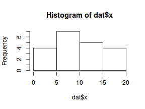
So lets explore linearity by creating a histogram of the predictor variable ($x$) and a scatterplot of the relationship between the response ($y$) and the predictor ($x$)
hist(dat$x)
# now for the scatterplot
plot(y ~ x, dat)
with(dat, lines(lowess(y ~ x)))
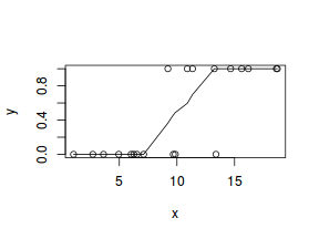
Conclusions: the predictor ($x$) does not display any skewness or other issues that might lead to non-linearity. The lowess smoother on the scatterplot does not display major deviations from a standard sigmoidal curve and thus linearity is satisfied. Violations of linearity could be addressed by either:
- define a non-linear linear predictor (such as a polynomial, spline or other non-linear function)
- transform the scale of the predictor variables
Model fitting or statistical analysis
There are a few of different functions and packages that we could use to fit a generalized linear model (or in this case a logist regression). Three of the most popular are:
- glm() from the stats package
- glmmTMB() from the glmmTMB package
- gamlss() from the gamlss package
We perform the logistic regression using the glm() function. The most important (=commonly used) parameters/arguments for logistic regression are:
- formula: the linear model relating the response variable to the linear predictor
- family: specification of the error distribution (and link function). Can be specified as either a string or as one of the family functions (which allows for the explicit declaration of the link function).
For examples:
- family="binomial" or equivalently family=binomial(link="logit")
- family=binomial(link="probit")
- data: the data frame containing the data
- weights: vector of weights to be used in the fitting process. These are particularly useful when dealing with grouped binary data from unequal sample sizes (see below).
I will demonstrate logistic regression with a range of possible link functions (each of which yield different parameter interpretations):
- logit
$$log\left(\frac{\pi}{1-\pi}\right)=\beta_0+\beta_1x_1+\epsilon_i, \hspace{1cm}\epsilon\sim Binom(\lambda)$$
dat.glmL <- glm(y ~ x, data = dat, family = "binomial")
- probit
$$\phi^{-1}\left(\pi\right)=\beta_0+\beta_1x_1+\epsilon_i, \hspace{1cm}\epsilon\sim Binom(\lambda)$$
dat.glmP <- glm(y ~ x, data = dat, family = binomial(link = "probit"))
- complimentary log-log
$$log(-log(1-\pi))=\beta_0+\beta_1x_1+\epsilon_i, \hspace{1cm}\epsilon\sim Binom(\lambda)$$
dat.glmC <- glm(y ~ x, data = dat, family = binomial(link = "cloglog"))
We perform the logistic regression using the glmmTMB() function. The most important (=commonly used) parameters/arguments for logistic regression are:
- formula: the linear model relating the response variable to the linear predictor
- family: specification of the error distribution (and link function). Can be specified as either a string or as one of the family functions (which allows for the explicit declaration of the link function).
For examples:
- family="binomial" or equivalently family=binomial(link="logit")
- family=binomial(link="probit")
- data: the data frame containing the data
- weights: vector of weights to be used in the fitting process. These are particularly useful when dealing with grouped binary data from unequal sample sizes (see below).
I will demonstrate logistic regression with a range of possible link functions (each of which yield different parameter interpretations):
- logit
$$log\left(\frac{\pi}{1-\pi}\right)=\beta_0+\beta_1x_1+\epsilon_i, \hspace{1cm}\epsilon\sim Binom(\lambda)$$
library(glmmTMB)
dat.glmmTMBL <- glmmTMB(y ~ x, data = dat, family = "binomial")
- probit
$$\phi^{-1}\left(\pi\right)=\beta_0+\beta_1x_1+\epsilon_i, \hspace{1cm}\epsilon\sim Binom(\lambda)$$
dat.glmmTMBP <- glmmTMB(y ~ x, data = dat, family = binomial(link = "probit"))
- complimentary log-log
$$log(-log(1-\pi))=\beta_0+\beta_1x_1+\epsilon_i, \hspace{1cm}\epsilon\sim Binom(\lambda)$$
dat.glmmTMBC <- glmmTMB(y ~ x, data = dat, family = binomial(link = "cloglog"))
We perform the logistic regression using the gamlss() function. The most important (=commonly used) parameters/arguments for logistic regression are:
- formula: the linear model relating the response variable to the linear predictor
- family: specification of the error distribution (and link function).
This is a different specification from glm() and supports a much wider variety of
families, including mixtures.
For examples:
- family=BI() or equivalently family=BI(mu.link="logit")
- family=BI(mu.link="probit")
- data: the data frame containing the data
- weights: vector of weights to be used in the fitting process. These are particularly useful when dealing with grouped binary data from unequal sample sizes (see below).
I will demonstrate logistic regression with a range of possible link functions (each of which yield different parameter interpretations):
- logit
$$log\left(\frac{\pi}{1-\pi}\right)=\beta_0+\beta_1x_1+\epsilon_i, \hspace{1cm}\epsilon\sim Binom(\lambda)$$
library(gamlss)
dat.gamlssL <- gamlss(y ~ x, data = dat, family = BI())
GAMLSS-RS iteration 1: Global Deviance = 11.6514
GAMLSS-RS iteration 2: Global Deviance = 11.6514
- probit
$$\phi^{-1}\left(\pi\right)=\beta_0+\beta_1x_1+\epsilon_i, \hspace{1cm}\epsilon\sim Binom(\lambda)$$
dat.gamlssP <- gamlss(y ~ x, data = dat, family = BI(mu.link = "probit"))
GAMLSS-RS iteration 1: Global Deviance = 11.4522
GAMLSS-RS iteration 2: Global Deviance = 11.4522
- complimentary log-log
$$log(-log(1-\pi))=\beta_0+\beta_1x_1+\epsilon_i, \hspace{1cm}\epsilon\sim Binom(\lambda)$$
dat.gamlssC <- gamlss(y ~ x, data = dat, family = BI(mu.link = "cloglog"))
GAMLSS-RS iteration 1: Global Deviance = 12.1082
GAMLSS-RS iteration 2: Global Deviance = 12.1082
Model evaluation
Prior to exploring the model parameters, it is prudent to confirm that the model did indeed fit the assumptions and was an appropriate fit to the data.
| Extractor | Description |
|---|---|
| residuals() | Extracts the residuals from the model |
| fitted() | Extracts the predicted (expected) response values (on the link scale) at the observed levels of the linear predictor |
| predict() | Extracts the predicted (expected) response values (on either the link, response or terms (linear predictor) scale) |
| coef() | Extracts the model coefficients |
| deviance() | Extracts the deviance from the model |
| AIC() | Extracts the Akaike's Information Criterion from the model |
| extractAIC() | Extracts the generalized Akaike's Information Criterion from the model |
| summary() | Summarizes the important output and characteristics of the model |
| anova() | Computes an analysis of deviance or log-likelihood ratio test (LRT) from the model |
| plot() | Generates a series of diagnostic plots from the model |
Lets explore the diagnostics - particularly the residuals
plot(dat.glmL)
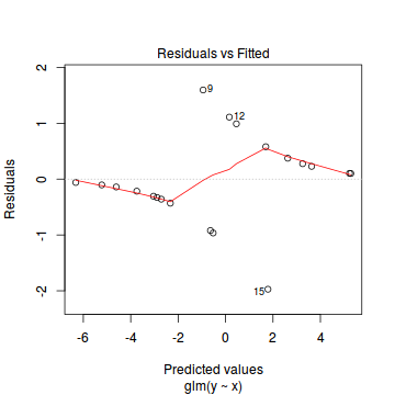
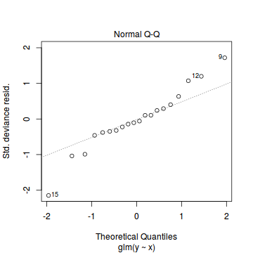
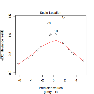
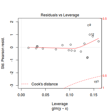
Unfortunately, unlike with linear models (Gaussian family), the expected distribution of data (residuals) varies over the range of fitted values for numerous (often competing) ways that make diagnosing (and attributing causes thereof) miss-specified generalized linear models from standard residual plots very difficult. The use of standardized (Pearson) residuals or deviance residuals can partly address this issue, yet they still do not offer completely consistent diagnoses across all issues (miss-specified model, over-dispersion, zero-inflation).
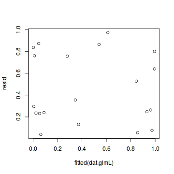
An alternative approach is to use simulated data from the fitted model to calculate an empirical cumulative density function from which residuals are are generated as values corresponding to the observed data along the density function. The (rather Bayesian) rationale is that if the model is correctly specified, then the observed data can be considered as a random draw from the fitted model. If this is the case, then residuals calculated from empirical cumulative density functions based on data simulated from the fitted model, should be totally uniform (flat) across the range of the linear predictor (fitted values) regardless of the model (Binomial, Poisson, linear, quadratic, hierarchical or otherwise). This uniformity can be explored by examining qq-plots (in which the trend should match a straight line) and plots of residual against the fitted values and each individual predictor (in which the noise should be uniform around zero across the range of x-values).
To illustrate this, lets generate 10 simulated data sets from our fitted model. This will generate a matrix with 10 columns and as many rows as there were in the original data. Think of it as 10 attempts to simulate the original data from the model.
dat.sim <- simulate(dat.glmL, n = 10)
dat.sim
   sim_1 sim_2 sim_3 sim_4 sim_5 sim_6 sim_7 sim_8 sim_9 sim_10
1      0     0     0     0     0     0     0     0     0      0
2      0     0     0     0     0     0     0     0     0      0
3      0     0     0     0     0     0     0     0     0      0
4      0     0     0     0     0     0     0     0     0      0
5      0     0     0     0     0     0     0     0     0      0
6      0     0     1     0     0     0     1     0     0      0
7      0     0     0     0     0     0     0     0     0      0
8      0     0     0     0     0     1     0     0     0      0
9      1     1     0     0     0     1     0     1     0      0
10     0     1     1     1     0     1     0     1     0      0
11     1     1     0     1     0     0     1     0     0      1
12     1     1     1     0     0     0     1     0     0      0
13     0     1     0     0     1     1     0     0     1      1
14     0     1     1     1     1     0     1     1     1      1
15     1     1     0     1     1     1     0     1     1      1
16     1     0     1     1     1     1     1     1     1      1
17     1     1     1     1     1     1     1     1     1      0
18     1     1     1     1     1     1     1     1     1      1
19     1     1     1     1     1     1     1     1     1      1
20     1     1     1     1     1     1     1     1     1      1
dat.sim <- simulate(dat.glmL, n = 250)
par(mfrow = c(5, 4), mar = c(3, 3, 1, 1))
resid <- NULL
for (i in 1:nrow(dat.sim)) {
    e = ecdf(data.matrix(dat.sim[i, ] + runif(250, -0.5, 0.5)))
    plot(e, main = i, las = 1)
    resid[i] <- e(dat$y[i] + runif(250, -0.5, 0.5))
}
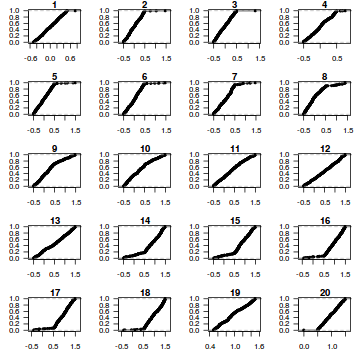
resid
 [1] 0.836 0.296 0.760 0.236 0.872 0.232 0.040 0.240 0.756 0.356 0.132 0.864 0.972 0.528 0.056 0.248
[17] 0.264 0.076 0.800 0.640
plot(resid ~ fitted(dat.glmL))
The DHARMa package provides a number of convenient routines to explore standardized residuals simulated from fitted models based on the concepts outlined above. Along with generating simulated residuals, simple qq plots and residual plots are available. By default, the residual plots include quantile regression lines (0.25, 0.5 and 0.75), each of which should be straight and flat.
- in overdispersed models, the qq trend will deviate substantially from a straight line
- non-linear models will display trends in the residuals
library(DHARMa)
dat.sim <- simulateResiduals(dat.glmL)
dat.sim
Object of Class DHARMa with simulated residuals based on 250 simulations with refit = FALSE . See ?DHARMa::simulateResiduals for help.

Scaled residual values: 0.492 0.664 0.216 0.952 0 0.84 0.592 0.66 0.988 0.48 0.456 0.9 0.596 0.692 0.028 0.988 0.944 0.456 0.436 0.176 ...
plotSimulatedResiduals(dat.sim)
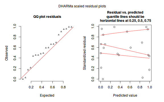
Conclusions: there is no obvious patterns in the qq-plot or residuals, or at least there are no obvious trends remaining that would be indicative of overdispersion or non-linearity.
We can also explore the goodness of the fit of the model via:
- Pearson's $\chi^2$ residuals
- explores whether there are any significant patterns remaining in the residuals
dat.resid <- sum(resid(dat.glmL, type = "pearson")^2)
1 - pchisq(dat.resid, dat.glmL$df.resid)
[1] 0.8571451
- Deviance ($G^2$) - similar to the $\chi^2$ test above, yet uses deviance
1 - pchisq(dat.glmL$deviance, dat.glmL$df.resid)
[1] 0.8647024
- The DHARMa package also has a routine for running a Kologorov-Smirnov test
test to explore overall uniformity of the residuals as a goodness-of-fit test on the scaled
residuals.
testUniformity(dat.sim)
	One-sample Kolmogorov-Smirnov test

data:  simulationOutput$scaledResiduals
D = 0.236, p-value = 0.2153
alternative hypothesis: two-sided
The DHARMa package also provides elegant ways to explore overdispersion, zero-inflation (and spatial and temporal autocorrelation). For these methods, the model is repeatedly refit with the simulated data to yield bootstrapped refitted residuals. The test for overdispersion compares the approximate deviances of the observed model with the those of the simulated models.
testOverdispersion(simulateResiduals(dat.glmL, refit = T))
	DHARMa nonparametric overdispersion test via comparison to simulation under H0 = fitted
	model

data:  simulateResiduals(dat.glmL, refit = T)
dispersion = 1.1716, p-value = 0.388
alternative hypothesis: overdispersion
testZeroInflation(simulateResiduals(dat.glmL, refit = T))
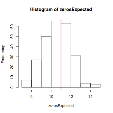
	DHARMa zero-inflation test via comparison to expected zeros with simulation under H0 =
	fitted model

data:  simulateResiduals(dat.glmL, refit = T)
ratioObsExp = 0.99171, p-value = 0.404
alternative hypothesis: more
In this demonstration, we fitted three logistic regressions (one for each link function). We could explore the residual plots of each of these for the purpose of comparing fit. We can also compare the fit of each of these three models via AIC (or deviance).
AIC(dat.glmL, dat.glmP, dat.glmC)
         df      AIC
dat.glmL  2 15.65141
dat.glmP  2 15.45223
dat.glmC  2 16.10823
| Extractor | Description |
|---|---|
| residuals() | Extracts the residuals from the model |
| fitted() | Extracts the predicted (expected) response values (on the link scale) at the observed levels of the linear predictor |
| predict() | Extracts the predicted (expected) response values (on either the link, response or terms (linear predictor) scale) |
| fixef() | Extracts the fixed model coefficients |
| AIC() | Extracts the Akaike's Information Criterion from the model |
| extractAIC() | Extracts the generalized Akaike's Information Criterion from the model |
| summary() | Summarizes the important output and characteristics of the model |
| confint() | Summarizes the important output and characteristics of the model |
| r2() | R-squared of the model |
Additional methods available can be explored via the following (substituting mod for the name of the fitted model).
methods(class=class(mod))
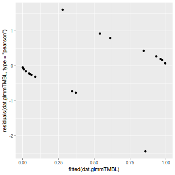
Lets explore the diagnostics - particularly the residuals
library(ggplot2)
ggplot(data = NULL) + geom_point(aes(y = residuals(dat.glmmTMBL, type = "pearson"), x = fitted(dat.glmmTMBL)))
qq.line = function(x) {
    # following four lines from base R's qqline()
    y <- quantile(x[!is.na(x)], c(0.25, 0.75))
    x <- qnorm(c(0.25, 0.75))
    slope <- diff(y)/diff(x)
    int <- y[1L] - slope * x[1L]
    return(c(int = int, slope = slope))
}
QQline = qq.line(resid(dat.glmmTMBL, type = "pearson"))
ggplot(data = NULL, aes(sample = resid(dat.glmmTMBL, type = "pearson"))) + stat_qq() + geom_abline(intercept = QQline[1],
    slope = QQline[2])
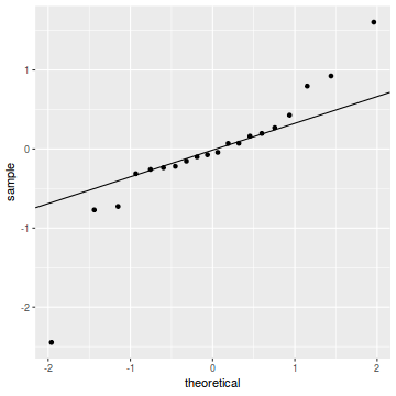
Unfortunately, unlike with linear models (Gaussian family), the expected distribution of data (residuals) varies over the range of fitted values for numerous (often competing) ways that make diagnosing (and attributing causes thereof) miss-specified generalized linear models from standard residual plots very difficult. The use of standardized (Pearson) residuals or deviance residuals can partly address this issue, yet they still do not offer completely consistent diagnoses across all issues (miss-specified model, over-dispersion, zero-inflation).
An alternative approach is to use simulated data from the fitted model to calculate an empirical cumulative density function from which residuals are are generated as values corresponding to the observed data along the density function. The (rather Bayesian) rationale is that if the model is correctly specified, then the observed data can be considered as a random draw from the fitted model. If this is the case, then residuals calculated from empirical cumulative density functions based on data simulated from the fitted model, should be totally uniform (flat) across the range of the linear predictor (fitted values) regardless of the model (Binomial, Poisson, linear, quadratic, hierarchical or otherwise). This uniformity can be explored by examining qq-plots (in which the trend should match a straight line) and plots of residual against the fitted values and each individual predictor (in which the noise should be uniform around zero across the range of x-values).
To illustrate this, lets generate 10 simulated data sets from our fitted model. This will generate a matrix with 10 columns and as many rows as there were in the original data. Think of it as 10 attempts to simulate the original data from the model.
dat.sim <- simulate(dat.glmmTMBL, n = 10)
dat.sim
   sim_1.1 sim_1.2 sim_2.1 sim_2.2 sim_3.1 sim_3.2 sim_4.1 sim_4.2 sim_5.1 sim_5.2 sim_6.1 sim_6.2
1        0       1       0       1       0       1       0       1       0       1       0       1
2        0       1       0       1       0       1       0       1       0       1       0       1
3        0       1       0       1       0       1       0       1       0       1       0       1
4        0       1       0       1       0       1       0       1       0       1       0       1
5        0       1       0       1       0       1       0       1       0       1       0       1
6        0       1       0       1       0       1       0       1       0       1       0       1
7        0       1       0       1       0       1       0       1       0       1       0       1
8        0       1       0       1       0       1       0       1       0       1       0       1
9        0       1       0       1       0       1       1       0       1       0       1       0
10       0       1       1       0       0       1       0       1       0       1       0       1
11       0       1       0       1       0       1       0       1       1       0       0       1
12       0       1       0       1       1       0       0       1       1       0       0       1
13       0       1       0       1       1       0       0       1       1       0       1       0
14       1       0       1       0       0       1       0       1       1       0       1       0
15       0       1       1       0       1       0       1       0       1       0       1       0
16       1       0       1       0       1       0       1       0       1       0       1       0
17       1       0       1       0       1       0       1       0       1       0       1       0
18       1       0       1       0       1       0       1       0       1       0       1       0
19       1       0       1       0       1       0       1       0       1       0       1       0
20       1       0       1       0       1       0       1       0       1       0       1       0
   sim_7.1 sim_7.2 sim_8.1 sim_8.2 sim_9.1 sim_9.2 sim_10.1 sim_10.2
1        0       1       0       1       0       1        0        1
2        0       1       0       1       0       1        0        1
3        0       1       0       1       0       1        0        1
4        0       1       0       1       0       1        0        1
5        0       1       0       1       0       1        0        1
6        0       1       0       1       0       1        0        1
7        0       1       0       1       0       1        0        1
8        0       1       0       1       0       1        0        1
9        0       1       1       0       0       1        0        1
10       0       1       1       0       0       1        0        1
11       0       1       1       0       1       0        0        1
12       0       1       1       0       1       0        0        1
13       0       1       1       0       0       1        0        1
14       1       0       0       1       1       0        1        0
15       1       0       1       0       1       0        0        1
16       1       0       1       0       1       0        1        0
17       1       0       1       0       1       0        1        0
18       1       0       1       0       1       0        1        0
19       1       0       1       0       1       0        1        0
20       1       0       1       0       1       0        1        0
For binomial glmmTMB models, there are two columns (one for success and one for failure) for each simulation. We only need one of these (the success field), so we will strip out every second column.
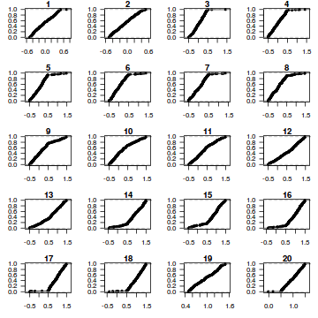
Now for each row of these simulated data, we calculate the empirical cumulative density function and use this function to predict new y-values (=residuals) corresponding to each observed y-value. Actually, 10 simulated samples is totally inadequate, we should use at least 250. I initially used 10, just so we could explore the output. We will re-simulate 250 times. Note also, for integer responses (including binary), uniform random noise is added to both the simulated and observed data so that we can sensibly explore zero inflation. The resulting residuals will be on a scale from 0 to 1 and therefore the residual plot should be centered around a y-value of 0.5.
dat.sim <- simulate(dat.glmmTMBL, n = 250)[, seq(1, 250 * 2, by = 2)]
par(mfrow = c(5, 4), mar = c(3, 3, 1, 1))
resid <- NULL
for (i in 1:nrow(dat.sim)) {
    e = ecdf(data.matrix(dat.sim[i, ] + runif(250, -0.5, 0.5)))
    plot(e, main = i, las = 1)
    resid[i] <- e(dat$y[i] + runif(250, -0.5, 0.5))
}
resid
 [1] 0.440 0.460 0.232 0.340 0.776 0.704 0.728 0.244 0.904 0.600 0.304 0.472 0.596 0.272 0.136 0.216
[17] 0.832 0.828 0.692 0.992
plot(resid ~ fitted(dat.glmmTMBL))
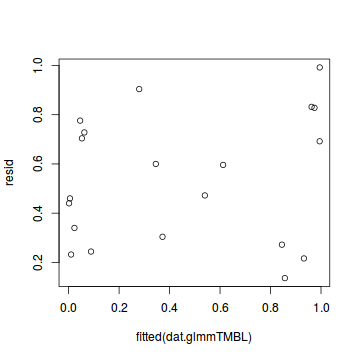
Conclusions: there is no obvious patterns in the qq-plot or residuals, or at least there are no obvious trends remaining that would be indicative of overdispersion or non-linearity.
We can also explore the goodness of the fit of the model via:
- Pearson's $\chi^2$ residuals
- explores whether there are any significant patterns remaining in the residuals
dat.resid <- sum(resid(dat.glmmTMBL, type = "pearson")^2)
1 - pchisq(dat.resid, df.residual(dat.glmmTMBL))
[1] 0.8571451
- Deviance ($G^2$) - similar to the $\chi^2$ test above, yet uses deviance
1 - pchisq(as.numeric(-2 * logLik(dat.glmmTMBL)), df.residual(dat.glmmTMBL))
[1] 0.8647024
In this demonstration, we fitted three logistic regressions (one for each link function). We could explore the residual plots of each of these for the purpose of comparing fit. We can also compare the fit of each of these three models via AIC (or deviance).
AIC(dat.glmmTMBL, dat.glmmTMBP, dat.glmmTMBC)
             df      AIC
dat.glmmTMBL  2 15.65141
dat.glmmTMBP  2 15.45223
dat.glmmTMBC  2 16.10823
| Extractor | Description |
|---|---|
| residuals() | Extracts the residuals from the model |
| fitted() | Extracts the predicted (expected) response values (on the link scale) at the observed levels of the linear predictor |
| predict() | Extracts the predicted (expected) response values (on either the link, response or terms (linear predictor) scale) |
| coef() | Extracts the model coefficients |
| deviance() | Extracts the deviance from the model |
| AIC() | Extracts the Akaike's Information Criterion from the model |
| extractAIC() | Extracts the generalized Akaike's Information Criterion from the model |
| summary() | Summarizes the important output and characteristics of the model |
| confint() | Summarizes the important output and characteristics of the model |
| Rsq() | R-squared of the model |
| plot() | Generates a series of diagnostic plots from the model |
Lets explore the diagnostics - particularly the residuals
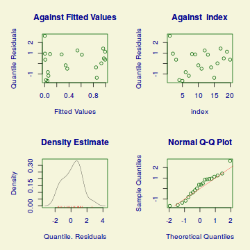
plot(dat.gamlssL)
******************************************************************
	 Summary of the Randomised Quantile Residuals
                           mean   =  0.1849072
                       variance   =  1.272725
               coef. of skewness  =  0.0372293
               coef. of kurtosis  =  2.229781
Filliben correlation coefficient  =  0.9830794
******************************************************************
Unfortunately, unlike with linear models (Gaussian family), the expected distribution of data (residuals) varies over the range of fitted values for numerous (often competing) ways that make diagnosing (and attributing causes thereof) miss-specified generalized linear models from standard residual plots very difficult. The use of standardized (Pearson) residuals or deviance residuals can partly address this issue, yet they still do not offer completely consistent diagnoses across all issues (miss-specified model, over-dispersion, zero-inflation).
Conclusions: there is no obvious patterns in the qq-plot or residuals, or at least there are no obvious trends remaining that would be indicative of overdispersion or non-linearity.
We can also explore the goodness of the fit of the model via:
- Pearson's $\chi^2$ residuals
- explores whether there are any significant patterns remaining in the residuals
dat.resid <- sum(resid(dat.gamlssL, type = "weighted", what = "mu")^2)
1 - pchisq(dat.resid, dat.gamlssL$df.resid)
[1] 0.8571451
- Deviance ($G^2$) - similar to the $\chi^2$ test above, yet uses deviance
1 - pchisq(deviance(dat.gamlssL), dat.gamlssL$df.resid)
[1] 0.8647024
In this demonstration, we fitted three logistic regressions (one for each link function). We could explore the residual plots of each of these for the purpose of comparing fit. We can also compare the fit of each of these three models via AIC (or deviance).
AIC(dat.gamlssL, dat.gamlssP, dat.gamlssC)
            df      AIC
dat.gamlssP  2 15.45223
dat.gamlssL  2 15.65141
dat.gamlssC  2 16.10823
Exploring partial effects plots
## using effects
library(effects)
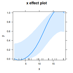
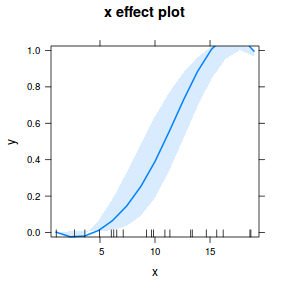
plot(allEffects(dat.glmL), type = "response")
library(sjPlot)
plot_model(dat.glmL, type = "pred", show.ci = TRUE, terms = "x")
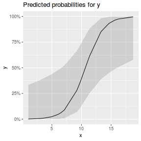
## using effects
library(effects)
plot(allEffects(dat.glmmTMBL), type = "response")
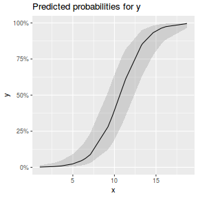
library(sjPlot)
plot_model(dat.glmmTMBL, type = "eff", show.ci = TRUE, terms = "x")
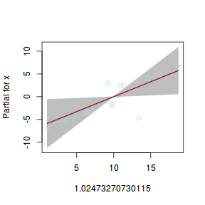
## using gamlss
term.plot(dat.gamlssL, x = x, se = T, partial = TRUE)
fittedPlot(dat.gamlssL, x = x)
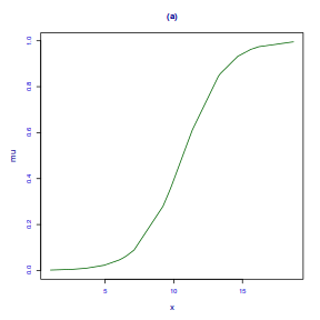
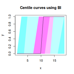
centiles.fan(dat.gamlssL, xvar = x)
## using effects
library(effects)
plot(allEffects(dat.gamlssL), type = "response")
Error in gamlss(formula = y ~ x, family = BI(), data = dat, method = "qr", : Method must be RS(), CG() or mixed()
library(sjPlot)
plot_model(dat.gamlssL, type = "pred", show.ci = TRUE, terms = "x")
Error in faminfo$family: $ operator is invalid for atomic vectors
Exploring the model parameters, test hypotheses
If there was any evidence that the assumptions had been violated or the model was not an appropriate fit, then we would need to reconsider the model and start the process again. In this case, there is no evidence that the test will be unreliable so we can proceed to explore the test statistics. The main statistic of interest is the Wald statistic ($z$) for the slope parameter.
summary(dat.glmL)
Call:
glm(formula = y ~ x, family = "binomial", data = dat)

Deviance Residuals:
     Min        1Q    Median        3Q       Max
-1.97157  -0.33665  -0.08191   0.30035   1.59628

Coefficients:
            Estimate Std. Error z value Pr(>|z|)
(Intercept)  -6.9899     3.1599  -2.212   0.0270 *
x             0.6559     0.2936   2.234   0.0255 *
---
Signif. codes:  0 '***' 0.001 '**' 0.01 '*' 0.05 '.' 0.1 ' ' 1

(Dispersion parameter for binomial family taken to be 1)

    Null deviance: 27.526  on 19  degrees of freedom
Residual deviance: 11.651  on 18  degrees of freedom
AIC: 15.651

Number of Fisher Scoring iterations: 6
exp(coef(dat.glmL))
(Intercept)           x
0.000921113 1.926780616
Conclusions:
- Intercept: when x is equal to zero, the odds of a success is
9 × 10⁻⁴times greater than the odds of failure. Or the corollary, the odds of a failure is1085.6432times greater than the odds of success. - Slope: for every 1 unit increase in x, the ratio odds of success to odds of failure changes by a factor of
1.9268. That is the odds ratio of success to failure nearly doubles with every 1 unit increase in x. From a inference testing perspective, we would reject the null hypothesis of no relationship.
summary(dat.glmmTMBL)
 Family: binomial  ( logit )
Formula:          y ~ x
Data: dat

     AIC      BIC   logLik deviance df.resid
    15.7     17.6     -5.8     11.7       18


Conditional model:
            Estimate Std. Error z value Pr(>|z|)
(Intercept)  -6.9899     3.1599  -2.212   0.0270 *
x             0.6559     0.2936   2.234   0.0255 *
---
Signif. codes:  0 '***' 0.001 '**' 0.01 '*' 0.05 '.' 0.1 ' ' 1
exp(fixef(dat.glmmTMBL)$cond)
 (Intercept)            x
0.0009211129 1.9267806990
Conclusions:
- Intercept: when x is equal to zero, the odds of a success is
9 × 10⁻⁴times greater than the odds of failure. Or the corollary, the odds of a failure is1085.6432times greater than the odds of success. - Slope: for every 1 unit increase in x, the ratio odds of success to odds of failure changes by a factor of
1.9268. That is the odds ratio of success to failure nearly doubles with every 1 unit increase in x. From a inference testing perspective, we would reject the null hypothesis of no relationship.
summary(dat.gamlssL)
******************************************************************
Family:  c("BI", "Binomial")

Call:  gamlss(formula = y ~ x, family = BI(), data = dat)

Fitting method: RS()

------------------------------------------------------------------
Mu link function:  logit
Mu Coefficients:
            Estimate Std. Error t value Pr(>|t|)
(Intercept)  -6.9899     3.1598  -2.212   0.0401 *
x             0.6559     0.2936   2.234   0.0384 *
---
Signif. codes:  0 '***' 0.001 '**' 0.01 '*' 0.05 '.' 0.1 ' ' 1

------------------------------------------------------------------
No. of observations in the fit:  20
Degrees of Freedom for the fit:  2
      Residual Deg. of Freedom:  18
                      at cycle:  2

Global Deviance:     11.65141
            AIC:     15.65141
            SBC:     17.64287
******************************************************************
exp(coef(dat.gamlssL))
(Intercept)           x
0.000921113 1.926780616
Conclusions:
- Intercept: when x is equal to zero, the odds of a success is
9 × 10⁻⁴times greater than the odds of failure. Or the corollary, the odds of a failure is1085.6432times greater than the odds of success. - Slope: for every 1 unit increase in x, the ratio odds of success to odds of failure changes by a factor of
1.9268. That is the odds ratio of success to failure nearly doubles with every 1 unit increase in x. From a inference testing perspective, we would reject the null hypothesis of no relationship.
Further explorations of the trends
A measure of the strength of the relationship can be obtained according to: $$quasi R^2 = 1-\left(\frac{deviance}{null~deviance}\right)$$
1 - (dat.glmL$deviance/dat.glmL$null)
[1] 0.5767057
1 - (as.numeric(-2 * logLik(dat.glmmTMBL))/as.numeric(-2 * logLik(update(dat.glmmTMBL,
    ~1))))
[1] 0.5767057
Rsq(dat.gamlssL)
[1] 0.5478346
We might also be interested in the LD50 - the value of $x$ where the probability switches from favoring 1 to favoring 0. LD50 is calculated as: $$LD50 = - \frac{intercept}{slope}$$
-dat.glmL$coef[1]/dat.glmL$coef[2]
(Intercept)
   10.65781
-fixef(dat.glmmTMBL)$cond[1]/fixef(dat.glmmTMBL)$cond[2]
(Intercept)
   10.65781
-coef(dat.gamlssL)[1]/coef(dat.gamlssL)[2]
(Intercept)
   10.65781
Logistic regression outcomes are often expressed in terms of odds ratios. Odds ratios are the ratio (or difference) of odds (which are themselves the ratio of the probability of one state to the probability of the alternate state) under two different scenarios. For example, the odds of the success/fail ratio when one condition is met vs when it is not met.
In Logistic regression, the parameters are on a log odds scale. Recall that the slope parameter of a model is typically interpreted as the change in expected response per unit change in predictor. Therefore, for logistic regression, the slope parameter represents the change (difference) on a log scale. Based on simple log laws, if we exponentiate this difference (slope), it becomes a division, and thus a ratio - a ratio of odds.
Alternatively, we could express this odds ratio in terms of relative risk. Whereas the odds ratio is the ratio of odds, relative risk is the ratio of probabilities. If risk is the probability of a state (probability of being absent), then we can express the effect of a treatment as the change in probability (risk) due to the treatment. This is the risk ratio and is calculated as: $$ R = \frac{OR}{(1+P_o+(P_o.OR)} $$ where $OR$ is the odd ratio and $P_o$ is the proportion of the incidence in the response - essentially the mean on the binary response.
exp(coef(dat.glmL)[2])
       x
1.926781
# Or for arbitrary unit changes
library(oddsratio)
## 1 unit change
or_glm(dat, dat.glmL, inc = list(x = 1))
  predictor oddsratio CI_low (2.5 %) CI_high (97.5 %) increment
1         x     1.927          1.278            4.551         1
## 5 units change
or_glm(dat, dat.glmL, inc = list(x = 5))
  predictor oddsratio CI_low (2.5 %) CI_high (97.5 %) increment
1         x    26.556          3.407         1951.831         5
## Alternatively, we could express this as relative risk RR <- OR / (1 - P0 + (P0 * OR)) where P0 is
## the proportion of incidence in response
sjstats::or_to_rr(exp(coef(dat.glmL)[2]), mean(model.frame(dat.glmL)[[1]]))
       x
1.359711
sjstats::odds_to_rr(dat.glmL)
                    RR     lower.ci  upper.ci
(Intercept) 0.00167349 1.814187e-07 0.1349919
x           1.35971129 1.135840e+00 1.7517501
- the odds ratio is
1.9267806. For a one unit increase in x, the odds of success nearly double. - the associated relative risk is
1.3597113. For a one unit increase in x, the probability of success increases by 36%. Every one unit change in x results in a 36% increase in risk of y being 1.
exp(fixef(dat.glmmTMBL)$cond[2])
       x
1.926781
## Alternatively, we could express this as relative risk RR <- OR / (1 - P0 + (P0 * OR)) where P0 is
## the proportion of incidence in response
sjstats::or_to_rr(exp(fixef(dat.glmmTMBL)$cond[2]), mean(model.frame(dat.glmmTMBL)[[1]]))
       x
1.359711
- the odds ratio is
1.9267806. For a one unit increase in x, the odds of success nearly double. - the associated relative risk is
1.3597113. For a one unit increase in x, the probability of success increases by 36%. Every one unit change in x results in a 36% increase in risk of y being 1.
exp(coef(dat.gamlssL)[2])
       x
1.926781
## Alternatively, we could express this as relative risk RR <- OR / (1 - P0 + (P0 * OR)) where P0 is
## the proportion of incidence in response
sjstats::or_to_rr(exp(coef(dat.gamlssL)[2]), mean(model.frame(dat.gamlssL)[[1]]))
       x
1.359711
- the odds ratio is
1.9267806. For a one unit increase in x, the odds of success nearly double. - the associated relative risk is
1.3597113. For a one unit increase in x, the probability of success increases by 36%. Every one unit change in x results in a 36% increase in risk of y being 1.
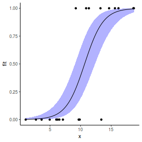
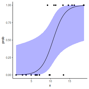
Finally, we will create a summary plot.
## using predict
newdata = with(dat, data.frame(x = seq(min(x), max(x), len = 100)))
fit = predict(dat.glmL, newdata = newdata, type = "link", se = TRUE)
q = qt(0.975, df = df.residual(dat.glmL))
newdata = cbind(newdata, fit = binomial()$linkinv(fit$fit),
    lower = binomial()$linkinv(fit$fit - q * fit$se.fit), upper = binomial()$linkinv(fit$fit +
        q * fit$se.fit))
ggplot(data = newdata, aes(y = fit, x = x)) + geom_point(data = dat,
    aes(y = y)) + geom_ribbon(aes(ymin = lower, ymax = upper),
    fill = "blue", alpha = 0.3) + geom_line() + theme_classic()

## using effects
library(effects)
xlevels = as.list(with(dat, data.frame(x = seq(min(x), max(x),
    len = 100))))
newdata = as.data.frame(Effect("x", dat.glmL, xlevels = xlevels))
ggplot(data = newdata, aes(y = fit, x = x)) + geom_point(data = dat,
    aes(y = y)) + geom_ribbon(aes(ymin = lower, ymax = upper),
    fill = "blue", alpha = 0.3) + geom_line() + theme_classic()
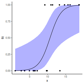
## using emmeans
library(emmeans)
newdata = with(dat, data.frame(x = seq(min(x), max(x), len = 100)))
newdata = summary(emmeans(ref_grid(dat.glmL, newdata), ~x),
    type = "response")
ggplot(data = newdata, aes(y = prob, x = x)) + geom_point(data = dat,
    aes(y = y)) + geom_ribbon(aes(ymin = asymp.LCL, ymax = asymp.UCL),
    fill = "blue", alpha = 0.3) + geom_line() + theme_classic()
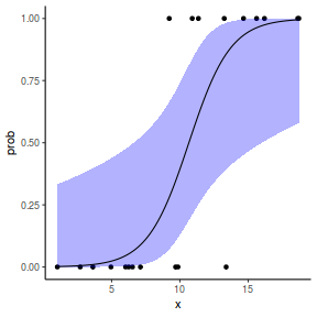
## or manually
newdata = with(dat, data.frame(x = seq(min(x), max(x), len = 100)))
Xmat = model.matrix(~x, data = newdata)
coefs = coef(dat.glmL)
fit = as.vector(coefs %*% t(Xmat))
se = sqrt(diag(Xmat %*% vcov(dat.glmL) %*% t(Xmat)))
q = qt(0.975, df = df.residual(dat.glmL))
newdata = cbind(newdata, fit = binomial()$linkinv(fit), lower = binomial()$linkinv(fit -
    q * se), upper = binomial()$linkinv(fit + q * se))
ggplot(data = newdata, aes(y = fit, x = x)) + geom_point(data = dat,
    aes(y = y)) + geom_ribbon(aes(ymin = lower, ymax = upper),
    fill = "blue", alpha = 0.3) + geom_line() + theme_classic()
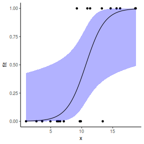
## using predict
newdata = with(dat, data.frame(x = seq(min(x), max(x), len = 100)))
fit = predict(dat.glmmTMBL, newdata = newdata, type = "link",
    se = TRUE)
q = qt(0.975, df = df.residual(dat.glmL))
newdata = cbind(newdata, fit = binomial()$linkinv(fit$fit),
    lower = binomial()$linkinv(fit$fit - q * fit$se.fit), upper = binomial()$linkinv(fit$fit +
        q * fit$se.fit))
ggplot(data = newdata, aes(y = fit, x = x)) + geom_point(data = dat,
    aes(y = y)) + geom_ribbon(aes(ymin = lower, ymax = upper),
    fill = "blue", alpha = 0.3) + geom_line() + theme_classic()

## using effects
library(effects)
xlevels = as.list(with(dat, data.frame(x = seq(min(x), max(x),
    len = 100))))
newdata = as.data.frame(Effect("x", dat.glmmTMBL, xlevels = xlevels))
ggplot(data = newdata, aes(y = fit, x = x)) + geom_point(data = dat,
    aes(y = y)) + geom_ribbon(aes(ymin = lower, ymax = upper),
    fill = "blue", alpha = 0.3) + geom_line() + theme_classic()
## using emmeans
library(emmeans)
newdata = with(dat, data.frame(x = seq(min(x), max(x), len = 100)))
newdata = summary(emmeans(ref_grid(dat.glmmTMBL, newdata),
    ~x), type = "response")
ggplot(data = newdata, aes(y = prob, x = x)) + geom_point(data = dat,
    aes(y = y)) + geom_ribbon(aes(ymin = lower.CL, ymax = upper.CL),
    fill = "blue", alpha = 0.3) + geom_line() + theme_classic()
## or manually
newdata = with(dat, data.frame(x = seq(min(x), max(x), len = 100)))
Xmat = model.matrix(~x, data = newdata)
coefs = fixef(dat.glmmTMBL)$cond
fit = as.vector(coefs %*% t(Xmat))
se = sqrt(diag(Xmat %*% vcov(dat.glmmTMBL)$cond %*% t(Xmat)))
q = qnorm(0.975)
newdata = cbind(newdata, fit = binomial()$linkinv(fit), lower = binomial()$linkinv(fit -
    q * se), upper = binomial()$linkinv(fit + q * se))
ggplot(data = newdata, aes(y = fit, x = x)) + geom_point(data = dat,
    aes(y = y)) + geom_ribbon(aes(ymin = lower, ymax = upper),
    fill = "blue", alpha = 0.3) + geom_line() + theme_classic()

## using predict - unfortunately, this still does not
## support se!

## using effects - not yet supported

## using emmeans
library(emmeans)
newdata = with(dat, data.frame(x = seq(min(x), max(x), len = 100)))
newdata = summary(emmeans(ref_grid(dat.gamlssL, newdata), ~x),
    type = "response")
ggplot(data = newdata, aes(y = response, x = x)) + geom_point(data = dat,
    aes(y = y)) + geom_ribbon(aes(ymin = asymp.LCL, ymax = asymp.UCL),
    fill = "blue", alpha = 0.3) + geom_line() + theme_classic()
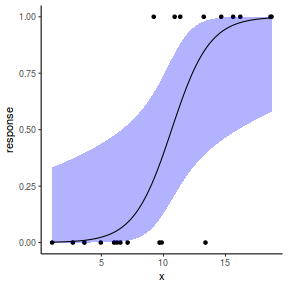
## or manually
newdata = with(dat, data.frame(x = seq(min(x), max(x), len = 100)))
Xmat = model.matrix(~x, data = newdata)
coefs = coef(dat.gamlssL)
fit = as.vector(coefs %*% t(Xmat))
se = sqrt(diag(Xmat %*% vcov(dat.gamlssL) %*% t(Xmat)))
q = qt(0.975, df = df.residual(dat.gamlssL))
newdata = cbind(newdata, fit = binomial()$linkinv(fit), lower = binomial()$linkinv(fit -
    q * se), upper = binomial()$linkinv(fit + q * se))
ggplot(data = newdata, aes(y = fit, x = x)) + geom_point(data = dat,
    aes(y = y)) + geom_ribbon(aes(ymin = lower, ymax = upper),
    fill = "blue", alpha = 0.3) + geom_line() + theme_classic()

Grouped binary data (and proportional data)
Scenario and Data
In the previous demonstration, the response variable represented the state of a single item per level of the predictor variable ($x$). That single item could be observed having a value of either 1 or 0. Another common situation is to observe the number of items in one of two states (typically dead or alive) for each level of a treatment. For example, you could tally up the number of germinated and non-germinated seeds out of a bank of 10 seeds at each of 8 temperature or nutrient levels.
Recall that the binomial distribution represents the density (probability) of all possible successes (germinations) out of a total of $N$ items (seeds). Hence the binomial distribution is also a suitable error distribution for such grouped binary data.
Similarly, proportional data (in which the response represents the frequency of events out of a set total of events) is also a good match for the binomial distribution. After all, the binomial distribution represents the distribution of successes out of a set number of trials. Examples of such data might be the proportion of female kangaroos with joey or the proportion of seeds taken by ants etc.
Indeed, binary data (ungrouped: presence/absence, dead/alive etc) is just a special case of proportional data in which the total (number of trials) in each case is 1. That is, the data are 1 out of 1 or 0 out of 1.
For this demonstration, we will model the number of successes against a uniformly distributed predictor ($x$). The number of trials in each group (level of the predictor) will vary slightly (yet randomly) so as to mimic complications that inevadably occur in real experiments.
- the number of levels of $x$ = 10
- the continuous $x$ variable is a random uniform spread of measurements between 10 and 20
- the rate of change in log odds ratio per unit change in x (slope) = -0.25. The magnitude of the slope is an indicator of how abruptly the log odds ratio changes. A very abrupt change would occur if there was very little variability in the trend. That is, a large slope would be indicative of a threshold effect. A lower slope indicates a gradual change in odds ratio and thus a less obvious and precise switch between the likelihood of 1 vs 0.
- the inflection point (point where the slope of the line is greatest) = 10. The inflection point indicates the value of the predictor ($x$) where the log Odds are 50% (switching between 1 being more likely and 0 being more likely). This is also known as the LD50.
- the intercept (which has no real interpretation) is equal to the negative of the slope multiplied by the inflection point
- generate the values of $y$ expected at each $x$ value, we evaluate the linear predictor.
- generate random numbers of trials per group by drawing integers out of a binomial distribution with a total size of 20 and probability of 0.9. Hence the maximum number of trials per group will be 20, yet some will be less than that.
- the number of success per group are drawn from a binomial distribution with a total size equal to the trial sizes generated in the previous step and probabilities equal to the expected $y$ values
- finally, the number of failures per group are calculated as the difference between the total trial size and number of successes per group.
set.seed(8)
# The number of levels of x
n.x <- 10
# Create x values that at uniformly distributed throughout the rate of 10 to 20
x <- sort(runif(n = n.x, min = 10, max = 20))
# The slope is the rate of change in log odds ratio for each unit change in x the smaller the slope,
# the slower the change (more variability in data too)
slope = -0.25
# Inflection point is where the slope of the line is greatest this is also the LD50 point
inflect <- 15
# Intercept (no interpretation)
intercept <- -1 * (slope * inflect)
# The linear predictor
linpred <- intercept + slope * x
# Predicted y values
y.pred <- exp(linpred)/(1 + exp(linpred))
# Add some noise and make binary (0's and 1's)
n.trial <- rbinom(n = n.x, 20, prob = 0.9)
success <- rbinom(n = n.x, size = n.trial, prob = y.pred)
failure <- n.trial - success
dat <- data.frame(success, failure, x)
Exploratory data analysis and initial assumption checking
- All of the observations are independent - this must be addressed at the design and collection stages
- The response variable (and thus the residuals) should be matched by an appropriate distribution (in the case of a binary response - a binomial is appropriate).
- All observations are equally influential in determining the trends - or at least no observations are overly influential. This is most effectively diagnosed via residuals and other influence indices and is very difficult to diagnose prior to analysis
- the relationship between the linear predictor (right hand side of the regression formula) and the link function should be linear. A scatterplot with smoother can be useful for identifying possible non-linearity.
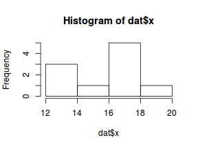
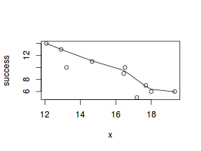
So lets explore linearity by creating a histogram of the predictor variable ($x$) and a scatterplot of the relationship between the either the number of successes ($success$) or the number of ($failures$) and the predictor ($x$). Note, that this will not account for the differences in trial size per group and so a scatterplot of the relationship between the number of successes ($success$) or the number of ($failures$) divided by the total number of trials against the predictor ($x$) might be more appropriate.
hist(dat$x)
# now for the scatterplot
plot(success ~ x, dat)
with(dat, lines(lowess(success ~ x)))
# scatterplot standardized for trial size
plot(success/(success + failure) ~ x, dat)
with(dat, lines(lowess(success/(success + failure) ~ x)))
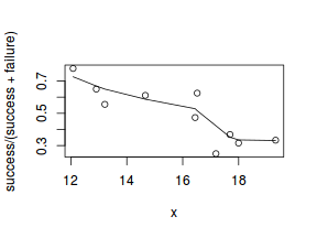
Conclusions: the predictor ($x$) does not display any skewness (although it is not all that uniform - random data hey!) or other issues that might lead to non-linearity. The lowess smoother on either scatterplot does not display major deviations from a standard sigmoidal curve and thus linearity is likely to be satisfied. Violations of linearity could be addressed by either:
- define a non-linear linear predictor (such as a polynomial, spline or other non-linear function)
- transform the scale of the predictor variables
Model fitting or statistical analysis
We perform the logistic regression using the glm() function. Clearly the number of successes is also dependent on the number of trials. Larger numbers of trials might be expected to yeild higher numbers of successes. Model weights can be used to account for differences in the total numbers of trials within each group. The most important (=commonly used) parameters/arguments for logistic regression are:
- formula: the linear model relating the response variable to the linear predictor
- family: specification of the error distribution (and link function). Can be specified as either a string or as one of the family functions (which allows for the explicit declaration of the link function).
For examples:
- family="binomial" or equivalently family=binomial(link="logit")
- family=binomial(link="probit")
- data: the data frame containing the data
- weights: vector of weights to be used in the fitting process. These are particularly useful when dealing with grouped binary data from unequal sample sizes.
I will demonstrate logistic regression with a range of possible link functions (each of which yield different parameter interpretations):
- logit
$$log\left(\frac{\pi}{1-\pi}\right)=\beta_0+\beta_1x_1+\epsilon_i, \hspace{1cm}\epsilon\sim Binom(\lambda)$$
dat.glmL <- glm(cbind(success, failure) ~ x, data = dat, family = "binomial")
# OR
dat <- within(dat, total <- success + failure)
dat.glmL <- glm(I(success/total) ~ x, data = dat, family = "binomial", weight = total)
- probit
$$\phi^{-1}\left(\pi\right)=\beta_0+\beta_1x_1+\epsilon_i, \hspace{1cm}\epsilon\sim Binom(\lambda)$$
dat.glmP <- glm(cbind(success, failure) ~ x, data = dat,
    family = binomial(link = "probit"))
# OR
dat <- within(dat, total <- success + failure)
dat.glmP <- glm(I(success/total) ~ x, data = dat, family = binomial(link = "probit"),
    weight = total)
- complimentary log-log
$$log(-log(1-\pi))=\beta_0+\beta_1x_1+\epsilon_i, \hspace{1cm}\epsilon\sim Binom(\lambda)$$
dat.glmC <- glm(cbind(success, failure) ~ x, data = dat,
    family = binomial(link = "cloglog"))
# OR
dat <- within(dat, total <- success + failure)
dat.glmC <- glm(I(success/total) ~ x, data = dat, family = binomial(link = "cloglog"),
    weight = total)
We perform the logistic regression using the glmmTMB() function. The most important (=commonly used) parameters/arguments for logistic regression are:
- formula: the linear model relating the response variable to the linear predictor
- family: specification of the error distribution (and link function). Can be specified as either a string or as one of the family functions (which allows for the explicit declaration of the link function).
For examples:
- family="binomial" or equivalently family=binomial(link="logit")
- family=binomial(link="probit")
- data: the data frame containing the data
- weights: vector of weights to be used in the fitting process. These are particularly useful when dealing with grouped binary data from unequal sample sizes (see below).
I will demonstrate logistic regression with a range of possible link functions (each of which yield different parameter interpretations):
- logit
$$log\left(\frac{\pi}{1-\pi}\right)=\beta_0+\beta_1x_1+\epsilon_i, \hspace{1cm}\epsilon\sim Binom(\lambda)$$
library(glmmTMB)
dat.glmmTMBL <- glmmTMB(cbind(success, failure) ~ x,
    data = dat, family = "binomial")
- probit
$$\phi^{-1}\left(\pi\right)=\beta_0+\beta_1x_1+\epsilon_i, \hspace{1cm}\epsilon\sim Binom(\lambda)$$
dat.glmmTMBP <- glmmTMB(cbind(success, failure) ~ x,
    data = dat, family = binomial(link = "probit"))
- complimentary log-log
$$log(-log(1-\pi))=\beta_0+\beta_1x_1+\epsilon_i, \hspace{1cm}\epsilon\sim Binom(\lambda)$$
dat.glmmTMBC <- glmmTMB(cbind(success, failure) ~ x,
    data = dat, family = binomial(link = "cloglog"))
We perform the logistic regression using the gamlss() function. The most important (=commonly used) parameters/arguments for logistic regression are:
- formula: the linear model relating the response variable to the linear predictor
- family: specification of the error distribution (and link function).
This is a different specification from glm() and supports a much wider variety of
families, including mixtures.
For examples:
- family=BI() or equivalently family=BI(mu.link="logit")
- family=BI(mu.link="probit")
- data: the data frame containing the data
- weights: vector of weights to be used in the fitting process. These are particularly useful when dealing with grouped binary data from unequal sample sizes (see below).
I will demonstrate logistic regression with a range of possible link functions (each of which yield different parameter interpretations):
- logit
$$log\left(\frac{\pi}{1-\pi}\right)=\beta_0+\beta_1x_1+\epsilon_i, \hspace{1cm}\epsilon\sim Binom(\lambda)$$
library(gamlss)
dat.gamlssL <- gamlss(cbind(success, failure) ~ x, data = dat,
    family = BI())
GAMLSS-RS iteration 1: Global Deviance = 38.6222
GAMLSS-RS iteration 2: Global Deviance = 38.6222
- probit
$$\phi^{-1}\left(\pi\right)=\beta_0+\beta_1x_1+\epsilon_i, \hspace{1cm}\epsilon\sim Binom(\lambda)$$
dat.gamlssP <- gamlss(cbind(success, failure) ~ x, data = dat,
    family = BI(mu.link = "probit"))
GAMLSS-RS iteration 1: Global Deviance = 38.6267
GAMLSS-RS iteration 2: Global Deviance = 38.6267
- complimentary log-log
$$log(-log(1-\pi))=\beta_0+\beta_1x_1+\epsilon_i, \hspace{1cm}\epsilon\sim Binom(\lambda)$$
dat.gamlssC <- gamlss(cbind(success, failure) ~ x, data = dat,
    family = BI(mu.link = "cloglog"))
GAMLSS-RS iteration 1: Global Deviance = 38.5955
GAMLSS-RS iteration 2: Global Deviance = 38.5955
Model evaluation
Prior to exploring the model parameters, it is prudent to confirm that the model did indeed fit the assumptions and was an appropriate fit to the data.
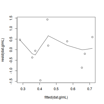
Lets explore the diagnostics - particularly the residuals
plot(resid(dat.glmL) ~ fitted(dat.glmL))
lines(lowess(resid(dat.glmL) ~ fitted(dat.glmL)))
dat.sim <- simulateResiduals(dat.glmL)
plotSimulatedResiduals(dat.sim)
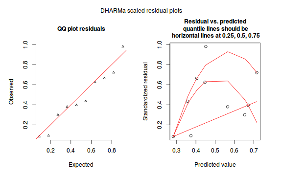
Conclusions: there is no obvious patterns in the residuals, or at least there are no obvious trends remaining that would be indicative of non-linearity.
We can also explore the goodness of the fit of the model via:
- Pearson's $\chi^2$ residuals
- explores whether there are any significant patterns remaining in the residuals
dat.resid <- sum(resid(dat.glmL, type = "pearson")^2)
1 - pchisq(dat.resid, dat.glmL$df.resid)
[1] 0.6763891
- Deviance ($G^2$) - similar to the $chi^2$ test above, yet uses deviance
1 - pchisq(dat.glmL$deviance, dat.glmL$df.resid)
[1] 0.6646471
- using the DHARMa package
testUniformity(dat.sim)
	One-sample Kolmogorov-Smirnov test

data:  simulationOutput$scaledResiduals
D = 0.18, p-value = 0.8473
alternative hypothesis: two-sided
In the absence of any evidence of a goodness of the fit of the model, there is unlikely to be any issues with overdispersion. However, it is worth estimating the dispersion parameter nonetheless.
- Pearson's $\chi^2$ residuals
- explores whether there are any significant patterns remaining in the residuals
dat.resid <- sum(resid(dat.glmL, type = "pearson")^2)
dat.resid/dat.glmL$df.resid
[1] 0.7174332
- Deviance ($G^2$) - similar to the $chi^2$ test above, yet uses deviance
dat.glmL$deviance/dat.glmL$df.resid
[1] 0.7305604
- using the DHARMa package
testOverdispersion(simulateResiduals(dat.glmL, refit = T))
Error in ecdf(out$refittedResiduals[i, ] + runif(out$nSim, -0.5, 0.5)): 'x' must have 1 or more non-missing values
testZeroInflation(simulateResiduals(dat.glmL, refit = T))
Error in ecdf(out$refittedResiduals[i, ] + runif(out$nSim, -0.5, 0.5)): 'x' must have 1 or more non-missing values
In this demonstration, we fitted three logistic regressions (one for each link function). We could explore the residual plots of each of these for the purpose of comparing fit. We can also compare the fit of each of these three models via AIC (or deviance).
AIC(dat.glm, dat.glmP, dat.glmC)
Error in AIC(dat.glm, dat.glmP, dat.glmC): object 'dat.glm' not found
library(ggplot2)
ggplot(data = NULL) + geom_point(aes(y = residuals(dat.glmmTMBL,
    type = "pearson"), x = fitted(dat.glmmTMBL)))
qq.line = function(x) {
    # following four lines from base R's qqline()
    y <- quantile(x[!is.na(x)], c(0.25, 0.75))
    x <- qnorm(c(0.25, 0.75))
    slope <- diff(y)/diff(x)
    int <- y[1L] - slope * x[1L]
    return(c(int = int, slope = slope))
}
QQline = qq.line(resid(dat.glmmTMBL, type = "pearson"))
ggplot(data = NULL, aes(sample = resid(dat.glmmTMBL, type = "pearson"))) +
    stat_qq() + geom_abline(intercept = QQline[1], slope = QQline[2])
dat.sim <- simulate(dat.glmmTMBL, n = 250)[, seq(1, 250 * 2,
    by = 2)]
par(mfrow = c(4, 3), mar = c(3, 3, 1, 1))
resid <- NULL
for (i in 1:nrow(dat.sim)) {
    e = ecdf(data.matrix(dat.sim[i, ] + runif(250, -0.5, 0.5)))
    plot(e, main = i, las = 1)
    resid[i] <- e(dat$success[i] + runif(250, -0.5, 0.5))
}
resid
[1] 0.756 0.364 0.172 0.596 0.572 0.920 0.040 0.492 0.344 0.632
plot(resid ~ fitted(dat.glmmTMBL))
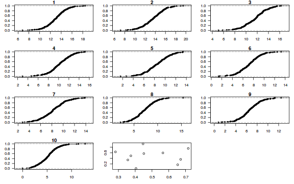
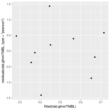
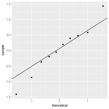
Conclusions: there is no obvious patterns in the residuals, or at least there are no obvious trends remaining that would be indicative of non-linearity.
We can also explore the goodness of the fit of the model via:
- Pearson's $\chi^2$ residuals
- explores whether there are any significant patterns remaining in the residuals
dat.resid <- sum(resid(dat.glmmTMBL, type = "pearson")^2)
1 - pchisq(dat.resid, df.residual(dat.glmmTMBL))
[1] 0.6763891
In the absence of any evidence of a goodness of the fit of the model, there is unlikely to be any issues with overdispersion. However, it is worth estimating the dispersion parameter nonetheless.
- Pearson's $\chi^2$ residuals
- explores whether there are any significant patterns remaining in the residuals
dat.resid <- sum(resid(dat.glmmTMBL, type = "pearson")^2)
dat.resid/df.residual(dat.glmmTMBL)
[1] 0.7174332
In this demonstration, we fitted three logistic regressions (one for each link function). We could explore the residual plots of each of these for the purpose of comparing fit. We can also compare the fit of each of these three models via AIC (or deviance).
AIC(dat.glmmTMBL, dat.glmmTMBP, dat.glmmTMBC)
             df      AIC
dat.glmmTMBL  2 42.62224
dat.glmmTMBP  2 42.62673
dat.glmmTMBC  2 42.59548
plot(dat.gamlssL)
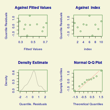
******************************************************************
	 Summary of the Randomised Quantile Residuals
                           mean   =  0.0461986
                       variance   =  0.4918538
               coef. of skewness  =  -0.04136291
               coef. of kurtosis  =  2.284877
Filliben correlation coefficient  =  0.9844053
******************************************************************
Unfortunately, unlike with linear models (Gaussian family), the expected distribution of data (residuals) varies over the range of fitted values for numerous (often competing) ways that make diagnosing (and attributing causes thereof) miss-specified generalized linear models from standard residual plots very difficult. The use of standardized (Pearson) residuals or deviance residuals can partly address this issue, yet they still do not offer completely consistent diagnoses across all issues (miss-specified model, over-dispersion, zero-inflation).
Conclusions: there is no obvious patterns in the qq-plot or residuals, or at least there are no obvious trends remaining that would be indicative of overdispersion or non-linearity.
We can also explore the goodness of the fit of the model via:
- Pearson's $\chi^2$ residuals
- explores whether there are any significant patterns remaining in the residuals
dat.resid <- sum(resid(dat.gamlssL, type = "weighted", what = "mu")^2)
1 - pchisq(dat.resid, dat.gamlssL$df.resid)
[1] 0.6763891
In this demonstration, we fitted three logistic regressions (one for each link function). We could explore the residual plots of each of these for the purpose of comparing fit. We can also compare the fit of each of these three models via AIC (or deviance).
AIC(dat.gamlssL, dat.gamlssP, dat.gamlssC)
            df      AIC
dat.gamlssC  2 42.59548
dat.gamlssL  2 42.62224
dat.gamlssP  2 42.62673
Exploring the model parameters, test hypotheses
If there was any evidence that the assumptions had been violated or the model was not an appropriate fit, then we would need to reconsider the model and start the process again. In this case, there is no evidence that the test will be unreliable so we can proceed to explore the test statistics. The main statistic of interest is the Wald statistic ($z$) for the slope parameter.
summary(dat.glmL)
Call:
glm(formula = I(success/total) ~ x, family = "binomial", data = dat,
    weights = total)

Deviance Residuals:
     Min        1Q    Median        3Q       Max
-1.45415  -0.32619   0.07158   0.45284   1.43145

Coefficients:
            Estimate Std. Error z value Pr(>|z|)
(Intercept)  4.01854    1.08802   3.693 0.000221 ***
x           -0.25622    0.06803  -3.766 0.000166 ***
---
Signif. codes:  0 '***' 0.001 '**' 0.01 '*' 0.05 '.' 0.1 ' ' 1

(Dispersion parameter for binomial family taken to be 1)

    Null deviance: 21.0890  on 9  degrees of freedom
Residual deviance:  5.8445  on 8  degrees of freedom
AIC: 42.622

Number of Fisher Scoring iterations: 3
exp(coef(dat.glmL))
(Intercept)           x
 55.6200133   0.7739699
library(broom)
tidy(dat.glmL)
# A tibble: 2 x 5
  term        estimate std.error statistic  p.value
  <chr>          <dbl>     <dbl>     <dbl>    <dbl>
1 (Intercept)    4.02     1.09        3.69 0.000221
2 x             -0.256    0.0680     -3.77 0.000166
glance(dat.glmL)
# A tibble: 1 x 7
  null.deviance df.null logLik   AIC   BIC deviance df.residual
          <dbl>   <int>  <dbl> <dbl> <dbl>    <dbl>       <int>
1          21.1       9  -19.3  42.6  43.2     5.84           8
Conclusions:
- Intercept: when x is equal to zero, the odds of a success is
55.62times greater than the odds of failure. - Slope: for every 1 unit increase in x, the ratio odds of success to odds of failure changes by a factor of
0.774. That is the odds ratio of success to failure declines at a rate of nearly 3/4 for every 1 unit increase in x. From a inference testing perspective, we would reject the null hypothesis of no relationship.
summary(dat.glmmTMBL)
 Family: binomial  ( logit )
Formula:          cbind(success, failure) ~ x
Data: dat

     AIC      BIC   logLik deviance df.resid
    42.6     43.2    -19.3     38.6        8


Conditional model:
            Estimate Std. Error z value Pr(>|z|)
(Intercept)  4.01854    1.08804   3.693 0.000221 ***
x           -0.25622    0.06803  -3.766 0.000166 ***
---
Signif. codes:  0 '***' 0.001 '**' 0.01 '*' 0.05 '.' 0.1 ' ' 1
exp(fixef(dat.glmmTMBL)$cond)
(Intercept)           x
 55.6200323   0.7739699
library(broom)
library(broom.mixed)  # devtools::install_github('bbolker/broom.mixed')
tidy(dat.glmmTMBL)
  effect component group        term   estimate  std.error statistic      p.value
1  fixed      cond fixed (Intercept)  4.0185434 1.08803755  3.693387 0.0002212871
2  fixed      cond fixed           x -0.2562223 0.06803094 -3.766261 0.0001657106
glance(dat.glmmTMBL)
  sigma    logLik      AIC      BIC df.residual
1     1 -19.31112 42.62224 43.22741           8
Conclusions:
- Intercept: when x is equal to zero, the odds of a success is
55.62times greater than the odds of failure. - Slope: for every 1 unit increase in x, the ratio odds of success to odds of failure changes by a factor of
0.774. That is the odds ratio of success to failure declines at a rate of nearly 3/4 for every 1 unit increase in x. From a inference testing perspective, we would reject the null hypothesis of no relationship.
summary(dat.gamlssL)
******************************************************************
Family:  c("BI", "Binomial")

Call:  gamlss(formula = cbind(success, failure) ~ x, family = BI(),      data = dat)

Fitting method: RS()

------------------------------------------------------------------
Mu link function:  logit
Mu Coefficients:
            Estimate Std. Error t value Pr(>|t|)
(Intercept)  4.01854    1.08805   3.693   0.0061 **
x           -0.25622    0.06803  -3.766   0.0055 **
---
Signif. codes:  0 '***' 0.001 '**' 0.01 '*' 0.05 '.' 0.1 ' ' 1

------------------------------------------------------------------
No. of observations in the fit:  10
Degrees of Freedom for the fit:  2
      Residual Deg. of Freedom:  8
                      at cycle:  2

Global Deviance:     38.62224
            AIC:     42.62224
            SBC:     43.22741
******************************************************************
exp(coef(dat.gamlssL))
(Intercept)           x
 55.6200134   0.7739699
library(broom)
tidy(dat.gamlssL)
  parameter        term   estimate std.error statistic     p.value
1        mu (Intercept)  4.0185431 1.0880241  3.693432 0.006099988
2        mu           x -0.2562222 0.0680295 -3.766340 0.005494302
glance(dat.gamlssL)
# A tibble: 1 x 6
     df logLik   AIC   BIC deviance df.residual
  <int>  <dbl> <dbl> <dbl>    <dbl>       <dbl>
1     0  -19.3  42.6  43.2     38.6          8.
Conclusions:
- Intercept: when x is equal to zero, the odds of a success is
55.62times greater than the odds of failure. - Slope: for every 1 unit increase in x, the ratio odds of success to odds of failure changes by a factor of
0.774. That is the odds ratio of success to failure declines at a rate of nearly 3/4 for every 1 unit increase in x. From a inference testing perspective, we would reject the null hypothesis of no relationship.
Further explorations of the trends
A measure of the strength of the relationship can be obtained according to: $$quasi R^2 = 1-\left(\frac{deviance}{null~deviance}\right)$$
1 - (dat.glmL$deviance/dat.glmL$null)
[1] 0.722866
We might also be interested in the LD50 - the value of $x$ where the probability switches from favoring 1 to favoring 0. LD50 is calculated as: $$LD50 = - \frac{intercept}{slope}$$
-dat.glmL$coef[1]/dat.glmL$coef[2]
(Intercept)
   15.68382
A measure of the strength of the relationship can be obtained according to: $$quasi R^2 = 1-\left(\frac{deviance}{null~deviance}\right)$$
1 - exp((2/nrow(dat)) * (logLik(update(dat.glmmTMBL, ~1))[1] - logLik(dat.glmmTMBL)[1]))
[1] 0.7822599
# This does not seem to work for proportional data.  The formula above relies on deviance being
# residual deviance that is -2*log(L/L_0) rather than -2*log(L)
1 - (as.numeric(-2 * logLik(dat.glmmTMBL))/as.numeric(-2 * logLik(update(dat.glmmTMBL, ~1))))
[1] 0.2830044
MuMIn::r.squaredGLMM(dat.glmmTMBL) # only seems to work when it is a mixed model
Error in reformulate(vapply(lapply(.findbars(form), "[[", 2L), deparse, : 'termlabels' must be a character vector of length at least one
We might also be interested in the LD50 - the value of $x$ where the probability switches from favoring 1 to favoring 0. LD50 is calculated as: $$LD50 = - \frac{intercept}{slope}$$
-fixef(dat.glmmTMBL)$cond[1]/fixef(dat.glmmTMBL)$cond[2]
(Intercept)
   15.68382
A measure of the strength of the relationship can be obtained according to: $$quasi R^2 = 1-\left(\frac{deviance}{null~deviance}\right)$$
Rsq(dat.gamlssL)
[1] 0.7822599
We might also be interested in the LD50 - the value of $x$ where the probability switches from favoring 1 to favoring 0. LD50 is calculated as: $$LD50 = - \frac{intercept}{slope}$$
-coef(dat.gamlssL)[1]/coef(dat.gamlssL)[2]
(Intercept)
   15.68382
Finally, we will create a summary plot.
# using predict
newdata = with(dat, data.frame(x = seq(min(x), max(x), len = 100)))
fit = predict(dat.glmL, newdata = newdata, type = "link", se = TRUE)
q = qt(0.975, df = df.residual(dat.glmL))
newdata = cbind(newdata, fit = binomial()$linkinv(fit$fit), lower = binomial()$linkinv(fit$fit -
    q * fit$se.fit), upper = binomial()$linkinv(fit$fit + q *
    fit$se.fit))
ggplot(data = newdata, aes(y = fit, x = x)) + geom_point(data = dat,
    aes(y = success/(success + failure))) + geom_ribbon(aes(ymin = lower,
    ymax = upper), fill = "blue", alpha = 0.3) + geom_line() +
    scale_y_continuous("Probability of success") + theme_classic()

## using effects
library(effects)
xlevels = as.list(with(dat, data.frame(x = seq(min(x), max(x),
    len = 100))))
newdata = as.data.frame(Effect("x", dat.glmL, xlevels = xlevels))
ggplot(data = newdata, aes(y = fit, x = x)) + geom_point(data = dat,
    aes(y = success/(success + failure))) + geom_ribbon(aes(ymin = lower,
    ymax = upper), fill = "blue", alpha = 0.3) + geom_line() +
    scale_y_continuous("Probability of success") + theme_classic()

## using emmeans
library(emmeans)
newdata = with(dat, data.frame(x = seq(min(x), max(x), len = 100)))
newdata = summary(emmeans(ref_grid(dat.glmL, newdata), ~x), type = "response")
ggplot(data = newdata, aes(y = prob, x = x)) + geom_point(data = dat,
    aes(y = success/(success + failure))) + geom_ribbon(aes(ymin = asymp.LCL,
    ymax = asymp.UCL), fill = "blue", alpha = 0.3) + geom_line() +
    scale_y_continuous("Probability of success") + theme_classic()
Error in FUN(X[[i]], ...): object 'prob' not found
## or manually
newdata = with(dat, data.frame(x = seq(min(x), max(x), len = 100)))
Xmat = model.matrix(~x, data = newdata)
coefs = coef(dat.glmL)
fit = as.vector(coefs %*% t(Xmat))
se = sqrt(diag(Xmat %*% vcov(dat.glmL) %*% t(Xmat)))
q = qt(0.975, df = df.residual(dat.glmL))
newdata = cbind(newdata, fit = binomial()$linkinv(fit), lower = binomial()$linkinv(fit -
    q * se), upper = binomial()$linkinv(fit + q * se))
ggplot(data = newdata, aes(y = fit, x = x)) + geom_point(data = dat,
    aes(y = success/(success + failure))) + geom_ribbon(aes(ymin = lower,
    ymax = upper), fill = "blue", alpha = 0.3) + geom_line() +
    scale_y_continuous("Probability of success") + theme_classic()

# using predict
newdata = with(dat, data.frame(x = seq(min(x), max(x), len = 100)))
fit = predict(dat.glmmTMBL, newdata = newdata, type = "link",
    se = TRUE)
q = qt(0.975, df = df.residual(dat.glmmTMBL))
newdata = cbind(newdata, fit = binomial()$linkinv(fit$fit), lower = binomial()$linkinv(fit$fit -
    q * fit$se.fit), upper = binomial()$linkinv(fit$fit + q *
    fit$se.fit))
ggplot(data = newdata, aes(y = fit, x = x)) + geom_point(data = dat,
    aes(y = success/(success + failure))) + geom_ribbon(aes(ymin = lower,
    ymax = upper), fill = "blue", alpha = 0.3) + geom_line() +
    scale_y_continuous("Probability of success") + theme_classic()

## using effects
library(effects)
xlevels = as.list(with(dat, data.frame(x = seq(min(x), max(x),
    len = 100))))
newdata = as.data.frame(Effect("x", dat.glmmTMBL, xlevels = xlevels))
ggplot(data = newdata, aes(y = fit, x = x)) + geom_point(data = dat,
    aes(y = success/(success + failure))) + geom_ribbon(aes(ymin = lower,
    ymax = upper), fill = "blue", alpha = 0.3) + geom_line() +
    scale_y_continuous("Probability of success") + theme_classic()

## using emmeans
library(emmeans)
newdata = with(dat, data.frame(x = seq(min(x), max(x), len = 100)))
newdata = summary(emmeans(ref_grid(dat.glmmTMBL, newdata), ~x),
    type = "response")
ggplot(data = newdata, aes(y = prob, x = x)) + geom_point(data = dat,
    aes(y = success/(success + failure))) + geom_ribbon(aes(ymin = lower.CL,
    ymax = upper.CL), fill = "blue", alpha = 0.3) + geom_line() +
    scale_y_continuous("Probability of success") + theme_classic()
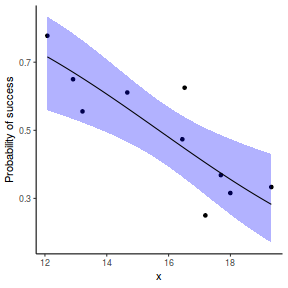
## or manually
newdata = with(dat, data.frame(x = seq(min(x), max(x), len = 100)))
Xmat = model.matrix(~x, data = newdata)
coefs = fixef(dat.glmmTMBL)$cond
fit = as.vector(coefs %*% t(Xmat))
se = sqrt(diag(Xmat %*% vcov(dat.glmmTMBL)$cond %*% t(Xmat)))
q = qnorm(0.975)
newdata = cbind(newdata, fit = binomial()$linkinv(fit), lower = binomial()$linkinv(fit -
    q * se), upper = binomial()$linkinv(fit + q * se))
ggplot(data = newdata, aes(y = fit, x = x)) + geom_point(data = dat,
    aes(y = success/(success + failure))) + geom_ribbon(aes(ymin = lower,
    ymax = upper), fill = "blue", alpha = 0.3) + geom_line() +
    scale_y_continuous("Probability of success") + theme_classic()
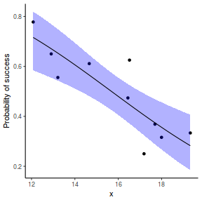
## using predict - unfortunately, this still does not support
## se!

## using effects - not yet supported

## using emmeans
library(emmeans)
newdata = with(dat, data.frame(x = seq(min(x), max(x), len = 100)))
newdata = summary(emmeans(ref_grid(dat.gamlssL, newdata), ~x),
    type = "response")
ggplot(data = newdata, aes(y = response, x = x)) + geom_point(data = dat,
    aes(y = success/(success + failure))) + geom_ribbon(aes(ymin = asymp.LCL,
    ymax = asymp.UCL), fill = "blue", alpha = 0.3) + geom_line() +
    scale_y_continuous("Probability of success") + theme_classic()

## or manually
newdata = with(dat, data.frame(x = seq(min(x), max(x), len = 100)))
Xmat = model.matrix(~x, data = newdata)
coefs = coef(dat.gamlssL)
fit = as.vector(coefs %*% t(Xmat))
se = sqrt(diag(Xmat %*% vcov(dat.gamlssL) %*% t(Xmat)))
q = qt(0.975, df = df.residual(dat.gamlssL))
newdata = cbind(newdata, fit = binomial()$linkinv(fit), lower = binomial()$linkinv(fit -
    q * se), upper = binomial()$linkinv(fit + q * se))
ggplot(data = newdata, aes(y = fit, x = x)) + geom_point(data = dat,
    aes(y = success/(success + failure))) + geom_ribbon(aes(ymin = lower,
    ymax = upper), fill = "blue", alpha = 0.3) + geom_line() +
    scale_y_continuous("Probability of success") + theme_classic()

Percentage data
Scenario and Data
In some ways, percentage data is similar to proportional data. In both cases, the expected values (ratio in the case of proportional data) are in the range from 0 to 1. However, the observations themselves have different geneses. For example, whereas for the proportional data, the observations (e.g. successes out of a total number of trials) are likely to be drawn from a binomial distribution, the same cannot be said for percentage data (as these are not counts).
Some modeling routines in R allow fractions to be modelled against a binomial distribution. Others are more strict and do not allow this. Arguably, percentage data is more appropriately modelled against a beta distribution.
For this simulated demonstration, lets assume that someone has designed a fairly simple linear regression experiment in which data are recorded along a perceived gradient in X. The measured response is the percent cover of some species. A total of 20 observations were observed.
- the number of levels of $x$ = 20
- the continuous $x$ variable is a random uniform spread of measurements between 1 and 20
- the rate of change in log odds ratio per unit change in x (slope) = 0.5. The magnitude of the slope is an indicator of how abruptly the log odds ratio changes. A very abrupt change would occur if there was very little variability in the trend. That is, a large slope would be indicative of a threshold effect. A lower slope indicates a gradual change in odds ratio and thus a less obvious and precise switch between the likelihood of 1 vs 0.
- the inflection point (point where the slope of the line is greatest) = 10. The inflection point indicates the value of the predictor ($x$) where the log Odds are 50% (switching between 1 being more likely and 0 being more likely). This is also known as the LD50.
- the intercept (which has no real interpretation) is equal to the negative of the slope multiplied by the inflection point
- generate the values of $y$ expected at each $x$ value, we evaluate the linear predictor.
- generate random numbers of trials per group by drawing integers out of a beta distribution with a total size of 20, shape1=$\alpha$ and shape2=$\beta$. We can express this relative to the linear predictor and some nominal $\sigma^2$ such that: $$ \begin{align} \mu &= \frac{\alpha}{\alpha+\beta}\\ \sigma^2 &= \frac{\alpha\beta}{(\alpha+\beta)^2 (\alpha+\beta+1)}\\ \end{align} $$ After a bit of rearranging, we observe that: $$ \begin{align} a &= \left(\frac{1-\mu}{\sigma^2} - \frac{1}{\mu}\right).\mu^2\\ b &= a\left(\frac{1}{\mu} - 1\right)\\ \end{align} $$
- the percent covers are drawn from a beta distribution
set.seed(8)
# The number of samples
n.x <- 20
# Create x values that at uniformly distributed throughout the rate of 1 to 20
x <- sort(runif(n = n.x, min = 1, max = 20))
# The slope is the rate of change in log odds ratio for each unit change in x the smaller the slope,
# the slower the change (more variability in data too)
slope = 0.5
# Inflection point is where the slope of the line is greatest this is also the LD50 point
inflect <- 10
# Intercept (no interpretation)
intercept <- -1 * (slope * inflect)
# The linear predictor
linpred <- intercept + slope * x
# Predicted y values
y.pred <- exp(linpred)/(1 + exp(linpred))
# Add some noise and make binomial
y.pred <- exp(linpred)/(1 + exp(linpred))
sigma = 0.01
estBetaParams <- function(mu, var) {
    alpha <- ((1 - mu)/var - 1/mu) * mu^2
    beta <- alpha * (1/mu - 1)
    return(params = list(alpha = alpha, beta = beta))
}
betaShapes = estBetaParams(y.pred, sigma)
y = rbeta(n = n.x, shape1 = betaShapes$alpha, shape2 = betaShapes$beta)
dat <- data.frame(y = round(y, 3), x)
Exploratory data analysis and initial assumption checking
- All of the observations are independent - this must be addressed at the design and collection stages
- The response variable (and thus the residuals) should be matched by an appropriate distribution (in the case of a percent cover response - a beta is appropriate).
One important consideration is that the beta distribution is defined in the range [0,1] but does not include 0 or 1. Often percentage data does have
0 or 1 values. If this is the case, there are a couple of options:
- convert values of 0 into something close to (yet slightly larger than 0) and do similar for values of 1.
- consider a zero-inflated beta (when there are values of zero), one-inflated beta (when there are values of one), or zero-one-inflated beta (when there are values of zero and one).
- All observations are equally influential in determining the trends - or at least no observations are overly influential. This is most effectively diagnosed via residuals and other influence indices and is very difficult to diagnose prior to analysis
- the relationship between the linear predictor (right hand side of the regression formula) and the link function should be linear. A scatterplot with smoother can be useful for identifying possible non-linearity.
So lets explore linearity by creating a histogram of the predictor variable ($x$) and a scatterplot of the relationship between the either the number of successes ($success$) or the number of ($failures$) and the predictor ($x$). Note, that this will not account for the differences in trial size per group and so a scatterplot of the relationship between the number of successes ($success$) or the number of ($failures$) divided by the total number of trials against the predictor ($x$) might be more appropriate.
hist(dat$x)

# now for the scatterplot
plot(y ~ x, dat)
with(dat, lines(lowess(y ~ x)))
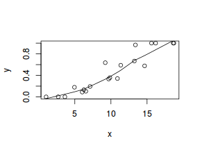
Conclusions: the predictor ($x$) does not display any skewness (although it is not all that uniform - random data hey!) or other issues that might lead to non-linearity. The lowess smoother on either scatterplot does not display major deviations from a standard sigmoidal curve and thus linearity is likely to be satisfied. Violations of linearity could be addressed by either:
- define a non-linear linear predictor (such as a polynomial, spline or other non-linear function)
- transform the scale of the predictor variables
Model fitting or statistical analysis
For the sake of comparison, we will fit this model using four different routines.
dat.glm <- glm(y ~ x, data = dat, family = "binomial")
library(betareg)
library(tidyverse)
dat = dat %>% mutate(y2 = ifelse(y == 0, 0.01, y), y2 = ifelse(y2 == 1, 0.99, y2))
dat.betareg <- betareg(y2 ~ x, data = dat)
library(glmmTMB)
dat = dat %>% mutate(y2 = ifelse(y == 0, 0.01, y), y2 = ifelse(y2 == 1, 0.99, y2))
dat.glmmTMB <- glmmTMB(y2 ~ x, data = dat, family = beta_family(link = "logit"))
library(gamlss)
dat.gamlss <- gamlss(y ~ x, data = dat, family = BEINF())
GAMLSS-RS iteration 1: Global Deviance = 9.6131
GAMLSS-RS iteration 2: Global Deviance = 8.0101
GAMLSS-RS iteration 3: Global Deviance = 7.9255
GAMLSS-RS iteration 4: Global Deviance = 7.9232
GAMLSS-RS iteration 5: Global Deviance = 7.9231
Model evaluation
Prior to exploring the model parameters, it is prudent to confirm that the model did indeed fit the assumptions and was an appropriate fit to the data.
Lets explore the diagnostics - particularly the residuals
plot(resid(dat.glm) ~ fitted(dat.glm))
lines(lowess(resid(dat.glm) ~ fitted(dat.glm)))
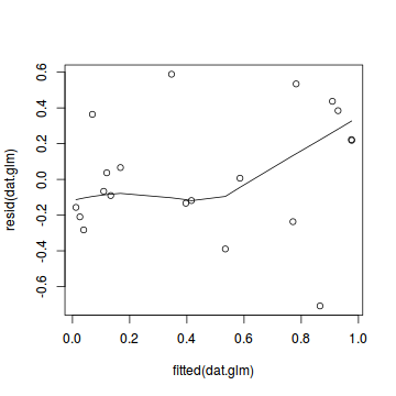
dat.sim <- simulateResiduals(dat.glm)
plotSimulatedResiduals(dat.sim)
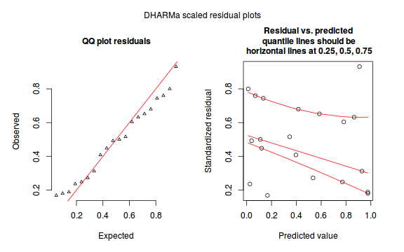
Conclusions: there is no obvious patterns in the residuals, or at least there are no obvious trends remaining that would be indicative of non-linearity.
We can also explore the goodness of the fit of the model via:
- Pearson's $\chi^2$ residuals
- explores whether there are any significant patterns remaining in the residuals
dat.resid <- sum(resid(dat.glm, type = "pearson")^2)
1 - pchisq(dat.resid, dat.glm$df.resid)
[1] 0.9999987
- Deviance ($G^2$) - similar to the $chi^2$ test above, yet uses deviance
1 - pchisq(dat.glm$deviance, dat.glm$df.resid)
[1] 0.9999983
- using the DHARMa package
testUniformity(dat.sim)
	One-sample Kolmogorov-Smirnov test

data:  simulationOutput$scaledResiduals
D = 0.168, p-value = 0.5681
alternative hypothesis: two-sided
In the absence of any evidence of a goodness of the fit of the model, there is unlikely to be any issues with overdispersion. However, it is worth estimating the dispersion parameter nonetheless.
- Pearson's $\chi^2$ residuals
- explores whether there are any significant patterns remaining in the residuals
dat.resid <- sum(resid(dat.glm, type = "pearson")^2)
dat.resid/dat.glm$df.resid
[1] 0.1131458
- Deviance ($G^2$) - similar to the $chi^2$ test above, yet uses deviance
dat.glm$deviance/dat.glm$df.resid
[1] 0.1172321
- using the DHARMa package
testOverdispersion(simulateResiduals(dat.glm, refit = T))
	DHARMa nonparametric overdispersion test via comparison to simulation under H0 = fitted
	model

data:  simulateResiduals(dat.glm, refit = T)
dispersion = 0.14353, p-value = 0.94
alternative hypothesis: overdispersion
testZeroInflation(simulateResiduals(dat.glm, refit = T))

	DHARMa zero-inflation test via comparison to expected zeros with simulation under H0 =
	fitted model

data:  simulateResiduals(dat.glm, refit = T)
ratioObsExp = 0.18484, p-value = 1
alternative hypothesis: more
plot(resid(dat.betareg) ~ fitted(dat.betareg))
lines(lowess(resid(dat.betareg) ~ fitted(dat.betareg)))
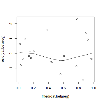
Conclusions: there is no obvious patterns in the residuals, or at least there are no obvious trends remaining that would be indicative of non-linearity.
We can also explore the goodness of the fit of the model via:
- Pearson's $\chi^2$ residuals
- explores whether there are any significant patterns remaining in the residuals
dat.resid <- sum(resid(dat.betareg, type = "pearson")^2)
1 - pchisq(dat.resid, dat.betareg$df.resid)
[1] 0.2952528
In the absence of any evidence of a goodness of the fit of the model, there is unlikely to be any issues with overdispersion. However, it is worth estimating the dispersion parameter nonetheless.
- Pearson's $\chi^2$ residuals
- explores whether there are any significant patterns remaining in the residuals
dat.resid <- sum(resid(dat.betareg, type = "pearson")^2)
dat.resid/dat.betareg$df.resid
[1] 1.152881
library(ggplot2)
ggplot(data = NULL) + geom_point(aes(y = residuals(dat.glmmTMB,
    type = "pearson"), x = fitted(dat.glmmTMB)))
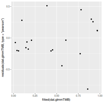
qq.line = function(x) {
    # following four lines from base R's qqline()
    y <- quantile(x[!is.na(x)], c(0.25, 0.75))
    x <- qnorm(c(0.25, 0.75))
    slope <- diff(y)/diff(x)
    int <- y[1L] - slope * x[1L]
    return(c(int = int, slope = slope))
}
QQline = qq.line(resid(dat.glmmTMB, type = "pearson"))
ggplot(data = NULL, aes(sample = resid(dat.glmmTMB, type = "pearson"))) +
    stat_qq() + geom_abline(intercept = QQline[1], slope = QQline[2])
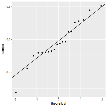
dat.sim <- simulate(dat.glmmTMB, n = 250)
par(mfrow = c(5, 4), mar = c(3, 3, 1, 1))
resid <- NULL
for (i in 1:nrow(dat.sim)) {
    e = ecdf(data.matrix(dat.sim[i, ] + runif(250, -0.5, 0.5)))
    plot(e, main = i, las = 1)
    resid[i] <- e(dat$y[i] + runif(250, -0.5, 0.5))
}
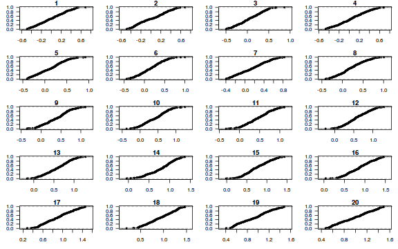
resid
 [1] 0.572 0.664 0.472 0.204 0.532 0.748 0.152 0.256 0.368 0.736 0.840 0.524 0.492 0.700 0.808 0.336
[17] 1.000 0.616 0.596 0.328
par(mfrow = c(1, 1))
plot(resid ~ fitted(dat.glmmTMB))
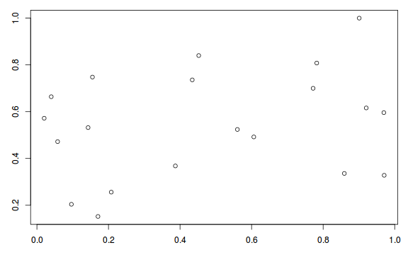
Conclusions: there is no obvious patterns in the residuals, or at least there are no obvious trends remaining that would be indicative of non-linearity.
We can also explore the goodness of the fit of the model via:
- Pearson's $\chi^2$ residuals
- explores whether there are any significant patterns remaining in the residuals
dat.resid <- sum(resid(dat.glmmTMB, type = "pearson")^2)
1 - pchisq(dat.resid, df.residual(dat.glmmTMB))
[1] 0.999998
In the absence of any evidence of a goodness of the fit of the model, there is unlikely to be any issues with overdispersion. However, it is worth estimating the dispersion parameter nonetheless.
- Pearson's $\chi^2$ residuals
- explores whether there are any significant patterns remaining in the residuals
dat.resid <- sum(resid(dat.glmmTMB, type = "pearson")^2)
dat.resid/df.residual(dat.glmmTMB)
[1] 0.1098094
plot(dat.gamlssL)

******************************************************************
	 Summary of the Randomised Quantile Residuals
                           mean   =  0.0461986
                       variance   =  0.4918538
               coef. of skewness  =  -0.04136291
               coef. of kurtosis  =  2.284877
Filliben correlation coefficient  =  0.9844053
******************************************************************
Conclusions: there is no obvious patterns in the qq-plot or residuals, or at least there are no obvious trends remaining that would be indicative of overdispersion or non-linearity.
We can also explore the goodness of the fit of the model via:
- Pearson's $\chi^2$ residuals
- explores whether there are any significant patterns remaining in the residuals
dat.resid <- sum(resid(dat.gamlssL, type = "weighted", what = "mu")^2)
1 - pchisq(dat.resid, dat.gamlssL$df.resid)
[1] 0.6763891
In the absence of any evidence of a goodness of the fit of the model, there is unlikely to be any issues with overdispersion. However, it is worth estimating the dispersion parameter nonetheless.
- Pearson's $\chi^2$ residuals
- explores whether there are any significant patterns remaining in the residuals
dat.resid <- sum(resid(dat.gamlss, type = "weighted", what = "mu")^2)
dat.resid/df.residual(dat.gamlss)
[1] 0.9089873
Exploring partial effects plots
## using effects
library(effects)
plot(allEffects(dat.glm), type = "response")
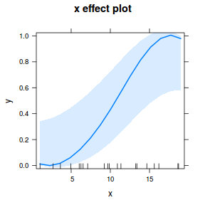
library(sjPlot)
plot_model(dat.glm, type = "pred", show.ci = TRUE, terms = "x")
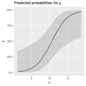
## using effects
library(effects)
plot(Effect("x", dat.betareg, xlevels = list(x = seq(min(dat$x),
    max(dat$x), len = 100))))
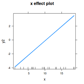
link = dat.betareg$link$mean
plot(allEffects(dat.betareg, type = "response", transform = list(trans = link$linkfun,
    inverse = link$linkinv)), type = "response")
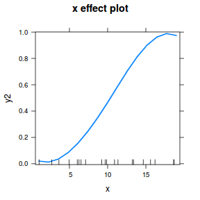
library(sjPlot)
plot_model(dat.betareg, type = "pred", show.ci = TRUE, terms = "x",
    transform = "binomial()$linkinv")
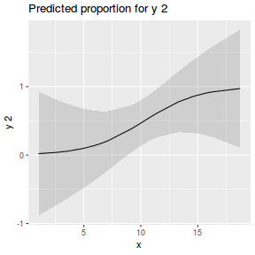
## using effects
library(effects)
plot(allEffects(dat.glmmTMB), type = "response")
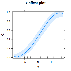
library(sjPlot)
plot_model(dat.glmmTMB, type = "eff", show.ci = TRUE, terms = "x")
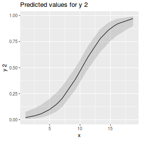
## using gamlss
term.plot(dat.gamlss, x = x, se = T, partial = TRUE)
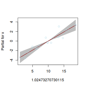
fittedPlot(dat.gamlss, x = x)
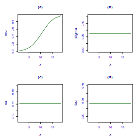
centiles.fan(dat.gamlss, xvar = x)
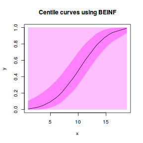
## using effects
library(effects)
plot(allEffects(dat.gamlss), type = "response")
Error in gamlss(formula = y ~ x, family = BEINF(), data = dat, method = "qr", : Method must be RS(), CG() or mixed()
library(sjPlot)
plot_model(dat.gamlss, type = "pred", show.ci = TRUE, terms = "x")
Error in faminfo$family: $ operator is invalid for atomic vectors
Exploring the model parameters, test hypotheses
If there was any evidence that the assumptions had been violated or the model was not an appropriate fit, then we would need to reconsider the model and start the process again. In this case, there is no evidence that the test will be unreliable so we can proceed to explore the test statistics. The main statistic of interest is the Wald statistic ($z$) for the slope parameter.
summary(dat.glm)
Call:
glm(formula = y ~ x, family = "binomial", data = dat)

Deviance Residuals:
     Min        1Q    Median        3Q       Max
-0.70852  -0.17005  -0.03006   0.25817   0.58884

Coefficients:
            Estimate Std. Error z value Pr(>|z|)
(Intercept)  -4.8626     2.0981  -2.318   0.0205 *
x             0.4588     0.1936   2.369   0.0178 *
---
Signif. codes:  0 '***' 0.001 '**' 0.01 '*' 0.05 '.' 0.1 ' ' 1

(Dispersion parameter for binomial family taken to be 1)

    Null deviance: 14.1513  on 19  degrees of freedom
Residual deviance:  2.1102  on 18  degrees of freedom
AIC: 13.985

Number of Fisher Scoring iterations: 5
binomial()$linkinv(coef(dat.glm))
(Intercept)           x
0.007671185 0.612720691
library(broom)
tidy(dat.glm)
# A tibble: 2 x 5
  term        estimate std.error statistic p.value
  <chr>          <dbl>     <dbl>     <dbl>   <dbl>
1 (Intercept)   -4.86      2.10      -2.32  0.0205
2 x              0.459     0.194      2.37  0.0178
glance(dat.glm)
# A tibble: 1 x 7
  null.deviance df.null logLik   AIC   BIC deviance df.residual
          <dbl>   <int>  <dbl> <dbl> <dbl>    <dbl>       <int>
1          14.2      19  -4.99  14.0  16.0     2.11          18
Conclusions:
- Intercept: when x is equal to zero, the estimated percent cover is
0.0077. - Slope: for every 1 unit increase in x, the percentage cover changes by
0.6127.
summary(dat.betareg)
Call:
betareg(formula = y2 ~ x, data = dat)

Standardized weighted residuals 2:
    Min      1Q  Median      3Q     Max
-1.7681 -0.5719 -0.2479  0.7006  2.2933

Coefficients (mean model with logit link):
            Estimate Std. Error z value Pr(>|z|)
(Intercept) -4.30109    0.50582  -8.503   <2e-16 ***
x            0.41680    0.04713   8.843   <2e-16 ***

Phi coefficients (precision model with identity link):
      Estimate Std. Error z value Pr(>|z|)
(phi)    9.499      3.163   3.003  0.00268 **
---
Signif. codes:  0 '***' 0.001 '**' 0.01 '*' 0.05 '.' 0.1 ' ' 1

Type of estimator: ML (maximum likelihood)
Log-likelihood: 27.05 on 3 Df
Pseudo R-squared: 0.8771
Number of iterations: 22 (BFGS) + 3 (Fisher scoring)
dat.betareg$link$mean$linkinv(coef(dat.betareg))
(Intercept)           x       (phi)
 0.01337254  0.60271817  0.99992507
library(broom)
tidy(dat.betareg)
# A tibble: 3 x 6
  component term        estimate std.error statistic  p.value
  <chr>     <chr>          <dbl>     <dbl>     <dbl>    <dbl>
1 mean      (Intercept)   -4.30     0.506      -8.50 1.84e-17
2 mean      x              0.417    0.0471      8.84 9.31e-19
3 precision (phi)          9.50     3.16        3.00 2.68e- 3
glance(dat.betareg)
# A tibble: 1 x 6
  pseudo.r.squared df.null logLik   AIC   BIC df.residual
             <dbl>   <dbl>  <dbl> <dbl> <dbl>       <int>
1            0.877     18.   27.0 -48.1 -45.1          17
Conclusions:
- Intercept: when x is equal to zero, the estimated percent cover is
0.0134. - Slope: for every 1 unit increase in x, the percentage cover changes by
0.6027.
summary(dat.glmmTMB)
 Family: beta  ( logit )
Formula:          y2 ~ x
Data: dat

     AIC      BIC   logLik deviance df.resid
   -48.1    -45.1     27.0    -54.1       17


Overdispersion parameter for beta family ():  9.5

Conditional model:
            Estimate Std. Error z value Pr(>|z|)
(Intercept) -4.30109    0.51895  -8.288   <2e-16 ***
x            0.41680    0.04792   8.699   <2e-16 ***
---
Signif. codes:  0 '***' 0.001 '**' 0.01 '*' 0.05 '.' 0.1 ' ' 1
family(dat.glmmTMB)$linkinv(fixef(dat.glmmTMB)$cond)
(Intercept)           x
 0.01337254  0.60271817
library(broom)
library(broom.mixed)  # devtools::install_github('bbolker/broom.mixed')
tidy(dat.glmmTMB)
  effect component group        term   estimate  std.error statistic      p.value
1  fixed      cond fixed (Intercept) -4.3010894 0.51894614 -8.288123 1.150497e-16
2  fixed      cond fixed           x  0.4168038 0.04791626  8.698587 3.360419e-18
glance(dat.glmmTMB)
    sigma   logLik       AIC       BIC df.residual
1 9.49893 27.04501 -48.09003 -45.10283          17
Conclusions:
- Intercept: when x is equal to zero, the estimated percent cover is
0.0077. - Slope: for every 1 unit increase in x, the percentage cover changes by
0.6127.
summary(dat.gamlss)
******************************************************************
Family:  c("BEINF", "Beta Inflated")

Call:  gamlss(formula = y ~ x, family = BEINF(), data = dat)

Fitting method: RS()

------------------------------------------------------------------
Mu link function:  logit
Mu Coefficients:
            Estimate Std. Error t value Pr(>|t|)
(Intercept) -4.03415    0.65895  -6.122 1.95e-05 ***
x            0.38129    0.06634   5.748 3.85e-05 ***
---
Signif. codes:  0 '***' 0.001 '**' 0.01 '*' 0.05 '.' 0.1 ' ' 1

------------------------------------------------------------------
Sigma link function:  logit
Sigma Coefficients:
            Estimate Std. Error t value Pr(>|t|)
(Intercept)  -0.7222     0.2464  -2.931   0.0103 *
---
Signif. codes:  0 '***' 0.001 '**' 0.01 '*' 0.05 '.' 0.1 ' ' 1

------------------------------------------------------------------
Nu link function:  log
Nu Coefficients:
            Estimate Std. Error t value Pr(>|t|)
(Intercept)  -1.9459     0.7559  -2.574   0.0212 *
---
Signif. codes:  0 '***' 0.001 '**' 0.01 '*' 0.05 '.' 0.1 ' ' 1

------------------------------------------------------------------
Tau link function:  log
Tau Coefficients:
            Estimate Std. Error t value Pr(>|t|)
(Intercept)  -1.2528     0.5669   -2.21   0.0431 *
---
Signif. codes:  0 '***' 0.001 '**' 0.01 '*' 0.05 '.' 0.1 ' ' 1

------------------------------------------------------------------
No. of observations in the fit:  20
Degrees of Freedom for the fit:  5
      Residual Deg. of Freedom:  15
                      at cycle:  5

Global Deviance:     7.92312
            AIC:     17.92312
            SBC:     22.90178
******************************************************************
binomial()$linkinv(coef(dat.gamlss)) # logit inverse
(Intercept)           x
 0.01739277  0.59418538
library(broom)
tidy(dat.gamlss)
  parameter        term   estimate  std.error statistic      p.value
1        mu (Intercept) -4.0341548 0.62893393 -6.414274 4.879024e-06
2        mu           x  0.3812949 0.06322293  6.030959 1.057823e-05
3     sigma (Intercept) -0.7222413 0.22820075 -3.164938 5.099291e-03
4        nu (Intercept) -1.9459101 0.74535591 -2.610713 1.718756e-02
5       tau (Intercept) -1.2527630 0.55901699 -2.241011 3.716592e-02
glance(dat.gamlss)
# A tibble: 1 x 6
     df logLik   AIC   BIC deviance df.residual
  <int>  <dbl> <dbl> <dbl>    <dbl>       <dbl>
1     0  -3.96  17.9  22.9     7.92         15.
Conclusions:
- Intercept: when x is equal to zero, the estimated percent cover is
0.0174. - Slope: for every 1 unit increase in x, the percentage cover changes by
0.5942.
Further explorations of the trends
A measure of the strength of the relationship can be obtained according to: $$quasi R^2 = 1-\left(\frac{deviance}{null~deviance}\right)$$
1 - (dat.glm$deviance/dat.glm$null)
[1] 0.8508845
0.851% of the variability in percent cover can be explained by its relationship to $x$.
dat.betareg$pseudo.r.squared
[1] 0.8771474
0.877% of the variability in percent cover can be explained by its relationship to $x$.
A measure of the strength of the relationship can be obtained according to: $$quasi R^2 = 1-\left(\frac{deviance}{null~deviance}\right)$$
1 - exp((2/nrow(dat)) * (logLik(update(dat.glmmTMB, ~1))[1] - logLik(dat.glmmTMB)[1]))
[1] 0.8679458
MuMIn::r.squaredGLMM(dat.glmmTMB) # only seems to work when it is a mixed model
Error in reformulate(vapply(lapply(.findbars(form), "[[", 2L), deparse, : 'termlabels' must be a character vector of length at least one
0.868% of the variability in presence/absence can be explained by its relationship to $x$.
Rsq(dat.gamlss)
[1] 0.6423063
0.642% of the variability in percent cover can be explained by its relationship to $x$.
Finally, we will create a summary plot.
# using predict
newdata = with(dat, data.frame(x = seq(min(x), max(x), len = 100)))
fit = predict(dat.glm, newdata = newdata, type = "link", se = TRUE)
q = qt(0.975, df = df.residual(dat.glm))
newdata = cbind(newdata, fit = binomial()$linkinv(fit$fit), lower = binomial()$linkinv(fit$fit -
    q * fit$se.fit), upper = binomial()$linkinv(fit$fit + q *
    fit$se.fit))
ggplot(data = newdata, aes(y = fit, x = x)) + geom_point(data = dat,
    aes(y = y)) + geom_ribbon(aes(ymin = lower, ymax = upper),
    fill = "blue", alpha = 0.3) + geom_line() + scale_y_continuous("Percentage cover") +
    theme_classic()
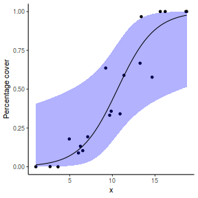
## using effects
library(effects)
xlevels = as.list(with(dat, data.frame(x = seq(min(x), max(x),
    len = 100))))
newdata = as.data.frame(Effect("x", dat.glm, xlevels = xlevels))
ggplot(data = newdata, aes(y = fit, x = x)) + geom_point(data = dat,
    aes(y = y)) + geom_ribbon(aes(ymin = lower, ymax = upper),
    fill = "blue", alpha = 0.3) + geom_line() + scale_y_continuous("Percentage cover") +
    theme_classic()

## using emmeans
library(emmeans)
newdata = with(dat, data.frame(x = seq(min(x), max(x), len = 100)))
newdata = summary(emmeans(ref_grid(dat.glm, newdata), ~x), type = "response")
ggplot(data = newdata, aes(y = prob, x = x)) + geom_point(data = dat,
    aes(y = y)) + geom_ribbon(aes(ymin = asymp.LCL, ymax = asymp.UCL),
    fill = "blue", alpha = 0.3) + geom_line() + scale_y_continuous("Percentage cover") +
    theme_classic()
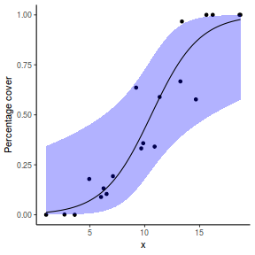
## or manually
newdata = with(dat, data.frame(x = seq(min(x), max(x), len = 100)))
Xmat = model.matrix(~x, data = newdata)
coefs = coef(dat.glm)
fit = as.vector(coefs %*% t(Xmat))
se = sqrt(diag(Xmat %*% vcov(dat.glm) %*% t(Xmat)))
q = qt(0.975, df = df.residual(dat.glm))
newdata = cbind(newdata, fit = binomial()$linkinv(fit), lower = binomial()$linkinv(fit -
    q * se), upper = binomial()$linkinv(fit + q * se))
ggplot(data = newdata, aes(y = fit, x = x)) + geom_point(data = dat,
    aes(y = y)) + geom_ribbon(aes(ymin = lower, ymax = upper),
    fill = "blue", alpha = 0.3) + geom_line() + scale_y_continuous("Percentage cover") +
    theme_classic()

# using predict - does not implement se
newdata = with(dat, data.frame(x = seq(min(x), max(x), len = 100)))
fit = predict(dat.betareg, newdata = newdata, type = "link",
    se = TRUE)
q = qt(0.975, df = df.residual(dat.betareg))
newdata = cbind(newdata, fit = binomial()$linkinv(fit))
ggplot(data = newdata, aes(y = fit, x = x)) + geom_point(data = dat,
    aes(y = y)) + geom_line() + scale_y_continuous("Percentage cover") +
    theme_classic()
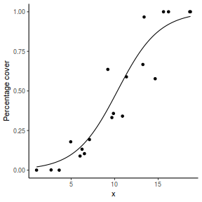
## using effects
library(effects)
xlevels = as.list(with(dat, data.frame(x = seq(min(x), max(x),
    len = 100))))
newdata = as.data.frame(Effect("x", dat.betareg, xlevels = xlevels,
    transform = list(trans = link$linkfun, inverse = link$linkinv)))
ggplot(data = newdata, aes(y = fit, x = x)) + geom_point(data = dat,
    aes(y = y)) + geom_ribbon(aes(ymin = lower, ymax = upper),
    fill = "blue", alpha = 0.3) + geom_line() + scale_y_continuous("Percentage cover") +
    theme_classic()
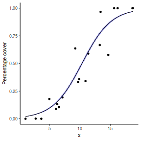
## using emmeans
library(emmeans)
newdata = with(dat, data.frame(x = seq(min(x), max(x), len = 100)))
newdata = summary(emmeans(ref_grid(dat.betareg, newdata), ~x),
    type = "response")
ggplot(data = newdata, aes(y = emmean, x = x)) + geom_point(data = dat,
    aes(y = y)) + geom_ribbon(aes(ymin = asymp.LCL, ymax = asymp.UCL),
    fill = "blue", alpha = 0.3) + geom_line() + scale_y_continuous("Percentage cover") +
    theme_classic()
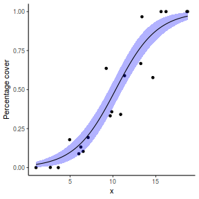
## or manually
newdata = with(dat, data.frame(x = seq(min(x), max(x), len = 100)))
Xmat = model.matrix(~x, data = newdata)
coefs = coef(dat.betareg)[-3]
fit = as.vector(coefs %*% t(Xmat))
se = sqrt(diag(Xmat %*% vcov(dat.betareg)[-3, -3] %*% t(Xmat)))
q = qt(0.975, df = df.residual(dat.betareg))
link = dat.betareg$link$mean
newdata = cbind(newdata, fit = link$linkinv(fit), lower = link$linkinv(fit -
    q * se), upper = link$linkinv(fit + q * se))
ggplot(data = newdata, aes(y = fit, x = x)) + geom_point(data = dat,
    aes(y = y)) + geom_ribbon(aes(ymin = lower, ymax = upper),
    fill = "blue", alpha = 0.3) + geom_line() + scale_y_continuous("Percentage cover") +
    theme_classic()

# using predict
newdata = with(dat, data.frame(x = seq(min(x), max(x), len = 100)))
fit = predict(dat.glmmTMB, newdata = newdata, type = "link",
    se = TRUE)
q = qt(0.975, df = df.residual(dat.glmmTMB))
newdata = cbind(newdata, fit = binomial()$linkinv(fit$fit), lower = binomial()$linkinv(fit$fit -
    q * fit$se.fit), upper = binomial()$linkinv(fit$fit + q *
    fit$se.fit))
ggplot(data = newdata, aes(y = fit, x = x)) + geom_point(data = dat,
    aes(y = y)) + geom_ribbon(aes(ymin = lower, ymax = upper),
    fill = "blue", alpha = 0.3) + geom_line() + scale_y_continuous("Percentage cover") +
    theme_classic()

## using effects
library(effects)
xlevels = as.list(with(dat, data.frame(x = seq(min(x), max(x),
    len = 100))))
newdata = as.data.frame(Effect("x", dat.glmmTMB, xlevels = xlevels))
ggplot(data = newdata, aes(y = fit, x = x)) + geom_point(data = dat,
    aes(y = y)) + geom_ribbon(aes(ymin = lower, ymax = upper),
    fill = "blue", alpha = 0.3) + geom_line() + scale_y_continuous("Percentage cover") +
    theme_classic()
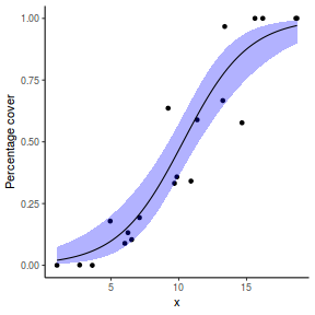
## using emmeans
library(emmeans)
newdata = with(dat, data.frame(x = seq(min(x), max(x), len = 100)))
newdata = summary(emmeans(ref_grid(dat.glmmTMB, newdata), ~x),
    type = "response")
ggplot(data = newdata, aes(y = prop, x = x)) + geom_point(data = dat,
    aes(y = y)) + geom_ribbon(aes(ymin = lower.CL, ymax = upper.CL),
    fill = "blue", alpha = 0.3) + geom_line() + scale_y_continuous("Percentage cover") +
    theme_classic()
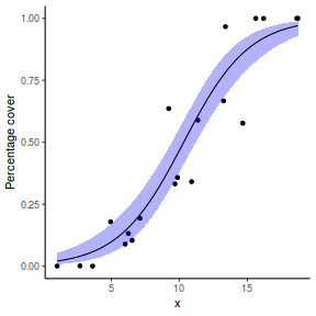
## or manually
newdata = with(dat, data.frame(x = seq(min(x), max(x), len = 100)))
Xmat = model.matrix(~x, data = newdata)
coefs = fixef(dat.glmmTMB)$cond
fit = as.vector(coefs %*% t(Xmat))
se = sqrt(diag(Xmat %*% vcov(dat.glmmTMB)$cond %*% t(Xmat)))
q = qnorm(0.975)
newdata = cbind(newdata, fit = binomial()$linkinv(fit), lower = binomial()$linkinv(fit -
    q * se), upper = binomial()$linkinv(fit + q * se))
ggplot(data = newdata, aes(y = fit, x = x)) + geom_point(data = dat,
    aes(y = y)) + geom_ribbon(aes(ymin = lower, ymax = upper),
    fill = "blue", alpha = 0.3) + geom_line() + scale_y_continuous("Percentage cover") +
    theme_classic()

## using predict - unfortunately, this still does not support
## se!

## using effects - not yet supported

## using emmeans
library(emmeans)
newdata = with(dat, data.frame(x = seq(min(x), max(x), len = 100)))
newdata = summary(emmeans(ref_grid(dat.gamlss, newdata), ~x),
    type = "response")
ggplot(data = newdata, aes(y = response, x = x)) + geom_point(data = dat,
    aes(y = y)) + geom_ribbon(aes(ymin = asymp.LCL, ymax = asymp.UCL),
    fill = "blue", alpha = 0.3) + geom_line() + scale_y_continuous("Percentage cover") +
    theme_classic()
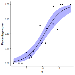
## or manually
newdata = with(dat, data.frame(x = seq(min(x), max(x), len = 100)))
Xmat = model.matrix(~x, data = newdata)
coefs = coef(dat.gamlss)
fit = as.vector(coefs %*% t(Xmat))
se = sqrt(diag(Xmat %*% vcov(dat.gamlss)[1:2, 1:2] %*% t(Xmat)))
q = qt(0.975, df = df.residual(dat.gamlss))
newdata = cbind(newdata, fit = binomial()$linkinv(fit), lower = binomial()$linkinv(fit -
    q * se), upper = binomial()$linkinv(fit + q * se))
ggplot(data = newdata, aes(y = fit, x = x)) + geom_point(data = dat,
    aes(y = y)) + geom_ribbon(aes(ymin = lower, ymax = upper),
    fill = "blue", alpha = 0.3) + geom_line() + scale_y_continuous("Percentage cover") +
    theme_classic()

Worked Examples
- Logan (2010) - Chpt 16-17
- Quinn & Keough (2002) - Chpt 13-14
Logistic regression
Polis et al. (1998) were intested in modelling the presence/absence of lizards (Uta sp.) against the perimeter to area ratio of 19 islands in the Gulf of California.
Download Polis data set| Format of polis.csv data file | |||||||||||||||||||||||||
|---|---|---|---|---|---|---|---|---|---|---|---|---|---|---|---|---|---|---|---|---|---|---|---|---|---|
|

|
polis <- read.table("../downloads/data/polis.csv", header = T, sep = ",", strip.white = T)
head(polis)
      ISLAND RATIO PA
1       Bota 15.41  1
2     Cabeza  5.63  1
3    Cerraja 25.92  1
4 Coronadito 15.17  0
5     Flecha 13.04  1
6   Gemelose 18.85  0
Presence absence data are clearly binary as an observation can only be in 1 of two states (1 or 0, present or absent). Modelling the linear component (systematic) against a normal stochastic component (that is expecting the residuals to follow a normal distribution) is clearly inappropriate. Instead, we could use a binary distribution with either a log link or probit link. For this example, we will use the log link and thus model the residuals on the log odds scale. In a later example, we will use the probit link.
- What is the null hypothesis of interest?
- Prior to fitting the model, we need to also be sure of the structure of the systematic linear component.
For example, is the relationship linear on the log odds scale?
Show code
plot(PA ~ RATIO, data = polis) with(polis, lines(lowess(PA ~ RATIO))) # check by fitting cubic spline library(splines) polis.glmS <- glm(PA ~ ns(RATIO), data = polis, family = "binomial") summary(polis.glmS)
Call: glm(formula = PA ~ ns(RATIO), family = "binomial", data = polis) Deviance Residuals: Min 1Q Median 3Q Max -1.6067 -0.6382 0.2368 0.4332 2.0986 Coefficients: Estimate Std. Error z value Pr(>|z|) (Intercept) 3.560 1.676 2.124 0.0336 * +\n s(RATIO) -17.238 7.892 -2.184 0.0289 * --- Signif. codes: 0 '***' 0.001 '**' 0.01 '*' 0.05 '.' 0.1 ' ' 1 (Dispersion parameter for binomial family taken to be 1) Null deviance: 26.287 on 18 degrees of freedom Residual deviance: 14.221 on 17 degrees of freedom AIC: 18.221 Number of Fisher Scoring iterations: 6xs <- with(polis, seq(min(RATIO), max(RATIO), l = 100)) ys <- predict(polis.glmS, newdata = data.frame(RATIO = xs), type = "response") lines(xs, ys, col = "red")

# The trend is more or less linear. If anything it is slightly sigmoidal yet so long as it is linear # within the bulk of the data, then linearity is fine.
-
Fitting the general linear model with a binomial error distribution (logit linkage)
(HINT).
Show glm code
polis.glm <- glm(PA ~ RATIO, family = binomial, data = polis)
Show glmmTMB codelibrary(glmmTMB) polis.glmmTMB <- glmmTMB(PA ~ RATIO, family = binomial, data = polis)
Show gamlss codelibrary(gamlss) polis.gamlss <- gamlss(PA ~ RATIO, family = BI(), data = polis)
GAMLSS-RS iteration 1: Global Deviance = 14.2207 GAMLSS-RS iteration 2: Global Deviance = 14.2207
- Check the model for lack of fit via:
- Pearson Χ2
Show glm code
polis.resid <- sum(resid(polis.glm, type = "pearson")^2) 1 - pchisq(polis.resid, polis.glm$df.resid)
[1] 0.5715331
# No evidence of a lack of fitShow glmmTMB codepolis.resid <- sum(resid(polis.glmmTMB, type = "pearson")^2) 1 - pchisq(polis.resid, df.residual(polis.glmmTMB))
[1] 0.571533
# No evidence of a lack of fitShow gamlss codepolis.resid <- sum(resid(polis.gamlss, type = "weighted", what = "mu")^2) 1 - pchisq(polis.resid, polis.gamlss$df.resid)
[1] 0.5715331
# No evidence of a lack of fit - Deviance (G2)
Show glm code
1 - pchisq(polis.glm$deviance, polis.glm$df.resid)
[1] 0.6514215
# No evidence of a lack of fitShow glmmTMB code1 - pchisq(as.numeric(-2 * logLik(polis.glmmTMB)), df.residual(polis.glmmTMB))
[1] 0.6514215
# No evidence of a lack of fitShow gamlss code1 - pchisq(deviance(polis.gamlss), polis.gamlss$df.resid)
[1] 0.6514215
# No evidence of a lack of fit - Explore the simulated residuals via the DHARMa package
Show glm code
library(DHARMa) polis.sim <- simulateResiduals(polis.glm) plotSimulatedResiduals(polis.sim)

testUniformity(polis.sim)
One-sample Kolmogorov-Smirnov test data: simulationOutput$scaledResiduals D = 0.16168, p-value = 0.7033 alternative hypothesis: two-sided
- Pearson Χ2
- Estimate the dispersion parameter to evaluate over dispersion in the fitted model
- Via Pearson residuals
Show glm code
polis.resid <- sum(resid(polis.glm, type = "pearson")^2) polis.resid/polis.glm$df.resid
[1] 0.9019219
# No evidence of over dispersionShow glmmTMB codepolis.resid <- sum(resid(polis.glmmTMB, type = "pearson")^2) polis.resid/df.residual(polis.glmmTMB)
[1] 0.9019219
# No evidence of over dispersionShow gamlss codepolis.resid <- sum(resid(polis.gamlss, type = "weighted", what = "mu")^2) polis.resid/polis.gamlss$df.residual
[1] 0.9019219
# No evidence of over dispersion - Via deviance
Show glm code
polis.glm$deviance/polis.glm$df.resid
[1] 0.8365126
# No evidence of over dispersionShow glmmTMB codeas.numeric(-2 * logLik(polis.glmmTMB))/df.residual(polis.glm)
[1] 0.8365126
# No evidence of over dispersionShow gamlss codedeviance(polis.gamlss)/polis.gamlss$df.resid
[1] 0.8365126
# No evidence of over dispersion - Explore the overdispersion via simulated residuals (DHARMa package)
Show code
library(DHARMa) polis.sim <- simulateResiduals(polis.glm, refit = T) testOverdispersion(polis.sim)
DHARMa nonparametric overdispersion test via comparison to simulation under H0 = fitted model data: polis.sim dispersion = 1.3051, p-value = 0.3 alternative hypothesis: overdispersion
- Via Pearson residuals
- Compare the expected number of zeros to the actual number of zeros to determine whether the model might be zero inflated.
- Calculate the proportion of zeros in the data
Show code
polis.tab <- table(polis$PA == 0) polis.tab/sum(polis.tab)
FALSE TRUE 0.5263158 0.4736842 - Assuming a probability of 0.5 for each trial, you would expect roughly 50:50 (50%) zeros and ones. So the data are not zero inflated.
- Calculate the proportion of zeros in the data
Show codelibrary(DHARMa) polis.sim <- simulateResiduals(polis.glm, refit = T) testZeroInflation(polis.sim)

DHARMa zero-inflation test via comparison to expected zeros with simulation under H0 = fitted model data: polis.sim ratioObsExp = 1.0195, p-value = 0.292 alternative hypothesis: more
- Check the model for lack of fit via:
-
As the parameterEstimates do not indicate any issues with the data or the fitted model, identify and interpret the following (HINT);
Show glm codepolis.glm <- glm(PA ~ RATIO, family = binomial, data = polis) summary(polis.glm)
Call: glm(formula = PA ~ RATIO, family = binomial, data = polis) Deviance Residuals: Min 1Q Median 3Q Max -1.6067 -0.6382 0.2368 0.4332 2.0986 Coefficients: Estimate Std. Error z value Pr(>|z|) (Intercept) 3.6061 1.6953 2.127 0.0334 * RATIO -0.2196 0.1005 -2.184 0.0289 * --- Signif. codes: 0 '***' 0.001 '**' 0.01 '*' 0.05 '.' 0.1 ' ' 1 (Dispersion parameter for binomial family taken to be 1) Null deviance: 26.287 on 18 degrees of freedom Residual deviance: 14.221 on 17 degrees of freedom AIC: 18.221 Number of Fisher Scoring iterations: 6library(broom) tidy(polis.glm)
# A tibble: 2 x 5 term estimate std.error statistic p.value <chr> <dbl> <dbl> <dbl> <dbl> 1 (Intercept) 3.61 1.70 2.13 0.0334 2 RATIO -0.220 0.101 -2.18 0.0289
glance(polis.glm)
# A tibble: 1 x 7 null.deviance df.null logLik AIC BIC deviance df.residual <dbl> <int> <dbl> <dbl> <dbl> <dbl> <int> 1 26.3 18 -7.11 18.2 20.1 14.2 17Show glmmTMB codesummary(polis.glmmTMB)
Family: binomial ( logit ) Formula: PA ~ RATIO Data: polis AIC BIC logLik deviance df.resid 18.2 20.1 -7.1 14.2 17 Conditional model: Estimate Std. Error z value Pr(>|z|) (Intercept) 3.6061 1.6952 2.127 0.0334 * RATIO -0.2196 0.1005 -2.184 0.0289 * --- Signif. codes: 0 '***' 0.001 '**' 0.01 '*' 0.05 '.' 0.1 ' ' 1library(broom) library(broom.mixed) # devtools::install_github('bbolker/broom.mixed') tidy(polis.glmmTMB)
effect component group term estimate std.error statistic p.value 1 fixed cond fixed (Intercept) 3.6060695 1.6952481 2.127163 0.03340652 2 fixed cond fixed RATIO -0.2195583 0.1005181 -2.184265 0.02894275
glance(polis.glmmTMB)
sigma logLik AIC BIC df.residual 1 1 -7.110357 18.22071 20.10959 17
Show gamlss codesummary(polis.gamlss)
****************************************************************** Family: c("BI", "Binomial") Call: gamlss(formula = PA ~ RATIO, family = BI(), data = polis) Fitting method: RS() ------------------------------------------------------------------ Mu link function: logit Mu Coefficients: Estimate Std. Error t value Pr(>|t|) (Intercept) 3.6061 1.6952 2.127 0.0483 * RATIO -0.2196 0.1005 -2.184 0.0432 * --- Signif. codes: 0 '***' 0.001 '**' 0.01 '*' 0.05 '.' 0.1 ' ' 1 ------------------------------------------------------------------ No. of observations in the fit: 19 Degrees of Freedom for the fit: 2 Residual Deg. of Freedom: 17 at cycle: 2 Global Deviance: 14.22071 AIC: 18.22071 SBC: 20.10959 ******************************************************************library(broom) tidy(polis.gamlss)
parameter term estimate std.error statistic p.value 1 mu (Intercept) 3.6060693 1.6952580 2.127151 0.04834506 2 mu RATIO -0.2195582 0.1005191 -2.184245 0.04324280
glance(polis.gamlss)
# A tibble: 1 x 6 df logLik AIC BIC deviance df.residual <int> <dbl> <dbl> <dbl> <dbl> <dbl> 1 0 -7.11 18.2 20.1 14.2 17.- sample constant (β0)
- sample slope (β1)
- Wald statistic (z value) for main H0
- P-value for main H0
- r2 value (HINT)
Show glm code
1 - (polis.glm$dev/polis.glm$null)
[1] 0.4590197
Show glmmTMB code1 - (as.numeric(-2 * logLik(polis.glmmTMB))/as.numeric(-2 * logLik(update(polis.glmmTMB, ~1))))
[1] 0.4590197
1 - exp((2/nrow(polis)) * (logLik(update(polis.glmmTMB, ~1))[1] - logLik(polis.glmmTMB)[1]))
[1] 0.4700986
Show gamlss codeRsq(polis.gamlss)
[1] 0.4700986
- sample constant (β0)
-
Another way ot test the fit of the model, and thus test the H0 that
β1 = 0, is to compare the fit of the full model to the reduce model via ANOVA.
Perform this ANOVA (HINT) and identify the following
Show codeanova(polis.glm, test = "Chisq")
Analysis of Deviance Table Model: binomial, link: logit Response: PA Terms added sequentially (first to last) Df Deviance Resid. Df Resid. Dev Pr(>Chi) NULL 18 26.287 RATIO 1 12.066 17 14.221 0.0005134 *** --- Signif. codes: 0 '***' 0.001 '**' 0.01 '*' 0.05 '.' 0.1 ' ' 1- G2 statistic
- df
- P value
- G2 statistic
- Construct a scatterplot of the presence/absence of Uta lizards against perimeter to area ratio for the 19 islands
(HINT).
Add to this plot, the predicted probability of occurances from the logistic regression (as well as 66% confidence interval - standard error).
(HINT)
Show glm code
## using predict newdata = with(polis, data.frame(RATIO = seq(min(RATIO), max(RATIO), len = 100))) fit = predict(polis.glm, newdata = newdata, type = "link", se = TRUE) q = qt(0.975, df = df.residual(polis.glm)) newdata = cbind(newdata, fit = binomial()$linkinv(fit$fit), lower = binomial()$linkinv(fit$fit - q * fit$se.fit), upper = binomial()$linkinv(fit$fit + q * fit$se.fit)) ggplot(data = newdata, aes(y = fit, x = RATIO)) + geom_point(data = polis, aes(y = PA)) + geom_ribbon(aes(ymin = lower, ymax = upper), fill = "blue", alpha = 0.3) + geom_line() + scale_y_continuous(expression(paste(italic(Uta), " lizard presence/absence"))) + scale_x_continuous("Island perimeter to area ratio") + theme_classic()

## using effects library(effects) xlevels = as.list(with(polis, data.frame(RATIO = seq(min(RATIO), max(RATIO), len = 100)))) newdata = as.data.frame(Effect("RATIO", polis.glm, xlevels = xlevels)) ggplot(data = newdata, aes(y = fit, x = RATIO)) + geom_point(data = polis, aes(y = PA)) + geom_ribbon(aes(ymin = lower, ymax = upper), fill = "blue", alpha = 0.3) + geom_line() + scale_y_continuous(expression(paste(italic(Uta), " lizard presence/absence"))) + scale_x_continuous("Island perimeter to area ratio") + theme_classic()

## using emmeans library(emmeans) newdata = with(polis, data.frame(RATIO = seq(min(RATIO), max(RATIO), len = 100))) newdata = summary(emmeans(ref_grid(polis.glm, newdata), ~RATIO), type = "response") ggplot(data = newdata, aes(y = prob, x = RATIO)) + geom_point(data = polis, aes(y = PA)) + geom_ribbon(aes(ymin = asymp.LCL, ymax = asymp.UCL), fill = "blue", alpha = 0.3) + geom_line() + scale_y_continuous(expression(paste(italic(Uta), " lizard presence/absence"))) + scale_x_continuous("Island perimeter to area ratio") + theme_classic()

## manually newdata = with(polis, data.frame(RATIO = seq(min(RATIO), max(RATIO), len = 100))) Xmat = model.matrix(~RATIO, data = newdata) coefs = coef(polis.glm) fit = as.vector(coefs %*% t(Xmat)) se = sqrt(diag(Xmat %*% vcov(polis.glm) %*% t(Xmat))) q = qt(0.975, df = df.residual(polis.glm)) newdata = cbind(newdata, fit = binomial()$linkinv(fit), lower = binomial()$linkinv(fit - q * se), upper = binomial()$linkinv(fit + q * se)) ggplot(data = newdata, aes(y = fit, x = RATIO)) + geom_point(data = polis, aes(y = PA)) + geom_ribbon(aes(ymin = lower, ymax = upper), fill = "blue", alpha = 0.3) + geom_line() + scale_y_continuous(expression(paste(italic(Uta), " lizard presence/absence"))) + scale_x_continuous("Island perimeter to area ratio") + theme_classic()
 Show glmmTMB code
## using predict newdata = with(polis, data.frame(RATIO = seq(min(RATIO), max(RATIO), len = 100))) fit = predict(polis.glmmTMB, newdata = newdata, type = "link", se = TRUE) q = qt(0.975, df = df.residual(polis.glmmTMB)) newdata = cbind(newdata, fit = binomial()$linkinv(fit$fit), lower = binomial()$linkinv(fit$fit - q * fit$se.fit), upper = binomial()$linkinv(fit$fit + q * fit$se.fit)) ggplot(data = newdata, aes(y = fit, x = RATIO)) + geom_point(data = polis, aes(y = PA)) + geom_ribbon(aes(ymin = lower, ymax = upper), fill = "blue", alpha = 0.3) + geom_line() + scale_y_continuous(expression(paste(italic(Uta), " lizard presence/absence"))) + scale_x_continuous("Island perimeter to area ratio") + theme_classic()

## using effects library(effects) xlevels = as.list(with(polis, data.frame(RATIO = seq(min(RATIO), max(RATIO), len = 100)))) newdata = as.data.frame(Effect("RATIO", polis.glmmTMB, xlevels = xlevels)) ggplot(data = newdata, aes(y = fit, x = RATIO)) + geom_point(data = polis, aes(y = PA)) + geom_ribbon(aes(ymin = lower, ymax = upper), fill = "blue", alpha = 0.3) + geom_line() + scale_y_continuous(expression(paste(italic(Uta), " lizard presence/absence"))) + scale_x_continuous("Island perimeter to area ratio") + theme_classic()

## using emmeans library(emmeans) newdata = with(polis, data.frame(RATIO = seq(min(RATIO), max(RATIO), len = 100))) newdata = summary(emmeans(ref_grid(polis.glmmTMB, newdata), ~RATIO), type = "response") ggplot(data = newdata, aes(y = prob, x = RATIO)) + geom_point(data = polis, aes(y = PA)) + geom_ribbon(aes(ymin = lower.CL, ymax = upper.CL), fill = "blue", alpha = 0.3) + geom_line() + scale_y_continuous(expression(paste(italic(Uta), " lizard presence/absence"))) + scale_x_continuous("Island perimeter to area ratio") + theme_classic()

## manually newdata = with(polis, data.frame(RATIO = seq(min(RATIO), max(RATIO), len = 100))) Xmat = model.matrix(~RATIO, data = newdata) coefs = fixef(polis.glmmTMB)$cond fit = as.vector(coefs %*% t(Xmat)) se = sqrt(diag(Xmat %*% vcov(polis.glmmTMB)$cond %*% t(Xmat))) q = qnorm(0.975) newdata = cbind(newdata, fit = binomial()$linkinv(fit), lower = binomial()$linkinv(fit - q * se), upper = binomial()$linkinv(fit + q * se)) ggplot(data = newdata, aes(y = fit, x = RATIO)) + geom_point(data = polis, aes(y = PA)) + geom_ribbon(aes(ymin = lower, ymax = upper), fill = "blue", alpha = 0.3) + geom_line() + scale_y_continuous(expression(paste(italic(Uta), " lizard presence/absence"))) + scale_x_continuous("Island perimeter to area ratio") + theme_classic()
 Show gamlss code
## using predict - unfortunately, this still does not support ## se! ## using effects - not yet supported ## using emmeans library(emmeans) newdata = with(polis, data.frame(RATIO = seq(min(RATIO), max(RATIO), len = 100))) newdata = summary(emmeans(ref_grid(polis.gamlss, newdata), ~RATIO), type = "response") ggplot(data = newdata, aes(y = response, x = RATIO)) + geom_point(data = polis, aes(y = PA)) + geom_ribbon(aes(ymin = asymp.LCL, ymax = asymp.UCL), fill = "blue", alpha = 0.3) + geom_line() + scale_y_continuous(expression(paste(italic(Uta), " lizard presence/absence"))) + scale_x_continuous("Island perimeter to area ratio") + theme_classic()

## manually newdata = with(polis, data.frame(RATIO = seq(min(RATIO), max(RATIO), len = 100))) Xmat = model.matrix(~RATIO, data = newdata) coefs = coef(polis.gamlss) fit = as.vector(coefs %*% t(Xmat)) se = sqrt(diag(Xmat %*% vcov(polis.gamlss) %*% t(Xmat))) q = qt(0.975, df = df.residual(polis.gamlss)) newdata = cbind(newdata, fit = binomial()$linkinv(fit), lower = binomial()$linkinv(fit - q * se), upper = binomial()$linkinv(fit + q * se)) ggplot(data = newdata, aes(y = fit, x = RATIO)) + geom_point(data = polis, aes(y = PA)) + geom_ribbon(aes(ymin = lower, ymax = upper), fill = "blue", alpha = 0.3) + geom_line() + scale_y_continuous(expression(paste(italic(Uta), " lizard presence/absence"))) + scale_x_continuous("Island perimeter to area ratio") + theme_classic()

-
Calculate the LD50 (in this case, the perimeter to area ratio with a predicted probability of 0.5) from the fitted model
(HINT).
Show glm code
-polis.glm$coef[1]/polis.glm$coef[2]
(Intercept) 16.4242Show glmmTMB code-fixef(polis.glmmTMB)$cond[1]/fixef(polis.glmmTMB)$cond[2]
(Intercept) 16.4242Show glmmTMB codeIslands above this ratio are not predicted to contain lizards and islands above this ratio are expected to have lizards.-coef(polis.gamlss)[1]/coef(polis.gamlss)[2]
(Intercept) 16.4242
- Examine the odds ratio for the occurrence of Uta lizards.
Show glm code
exp(coef(polis.glm)[2])
RATIO 0.8028734
# OR for arbitrary unit changes library(oddsratio) or_glm(polis, polis.glm, inc = list(RATIO = 1))
predictor oddsratio CI_low (2.5 %) CI_high (97.5 %) increment 1 RATIO 0.803 0.616 0.936 1
# the chances of Uta lizards being present on an island declines by approximately 20% (a change # factor of 0.803) for every unit increase in perimeter to area ratio. or_glm(polis, polis.glm, inc = list(RATIO = 10))
predictor oddsratio CI_low (2.5 %) CI_high (97.5 %) increment 1 RATIO 0.111 0.008 0.514 10
# the chances of Uta lizards being present on an island declines by approximately 90% (a change # factor of 0.111) for every 10 units increase in perimeter to area ratio. ## Alternatively, we could express this as relative risk RR <- OR / (1 - P0 + (P0 * OR)) where P0 is ## the proportion of incidence in response sjstats::or_to_rr(exp(coef(polis.glm)[2]), mean(model.frame(polis.glm)[[1]]))
RATIO 0.895815
sjstats::odds_to_rr(polis.glm)
RR lower.ci upper.ci (Intercept) 1.854667 1.4295083 1.8994502 RATIO 0.895815 0.7718324 0.9684614
Show glmmTMB codeexp(fixef(polis.glmmTMB)$cond[2])
RATIO 0.8028734
## Alternatively, we could express this as relative risk RR <- OR / (1 - P0 + (P0 * OR)) where P0 is ## the proportion of incidence in response sjstats::or_to_rr(exp(fixef(polis.glmmTMB)$cond[2]), mean(model.frame(polis.glmmTMB)[[1]]))
RATIO 0.8958149
Show gamlss codeexp(coef(polis.gamlss)[2])
RATIO 0.8028734
## Alternatively, we could express this as relative risk RR <- OR / (1 - P0 + (P0 * OR)) where P0 is ## the proportion of incidence in response sjstats::or_to_rr(exp(coef(polis.gamlss)[2]), mean(model.frame(polis.gamlss)[[1]]))
RATIO 0.895815
The chances of Uta lizards being present on an island declines by approximately 20% (a change factor of 0.803) for every unit increase in perimeter to area ratio. For every one unit increase in perimeter to area ratio, the risk of uta lizards being absent increases by
11.63% (1/0.896).
Logistic regression - grouped binary data
Bliss (1935) examined the toxic effects of gaseous carbon disulphide on the survival of flour beetles. He presented a number of datasets and associated analyses as a means to demonstrate models for calculating dosage curves.
In the first dataset, rather than indicating whether any individual beetle was dead or alive, Bliss (1935) recorded the number of dead and alive beetles grouped by gaseous carbon disulphide concentration.
Download the Bliss1 data set| Format of bliss1.csv data file | |||||||||||||||||||||||||
|---|---|---|---|---|---|---|---|---|---|---|---|---|---|---|---|---|---|---|---|---|---|---|---|---|---|
|

|
bliss <- read.table("../downloads/data/bliss1.csv", header = T, sep = ",", strip.white = T) head(bliss)
dead alive conc 1 2 28 0 2 8 22 1 3 15 15 2 4 23 7 3 5 27 3 4
- This is another example of clearly binary data (albeit in a different form).
There are three obvious link function worth trying
- log-link (the default)
Show glm code
bliss.glm <- glm(cbind(dead, alive) ~ conc, data = bliss, family = "binomial")
Show glmmTMB codelibrary(glmmTMB) bliss.glmmTMB <- glmmTMB(cbind(dead, alive) ~ conc, data = bliss, family = "binomial")
Show gamlss codelibrary(gamlss) bliss.gamlss <- gamlss(cbind(dead, alive) ~ conc, data = bliss, family = BI())
GAMLSS-RS iteration 1: Global Deviance = 16.854 GAMLSS-RS iteration 2: Global Deviance = 16.854
- probit
Show code
bliss.glmP <- glm(cbind(dead, alive) ~ conc, data = bliss, family = binomial(link = "probit"))
Show glmmTMB codelibrary(glmmTMB) bliss.glmmTMBC <- glmmTMB(cbind(dead, alive) ~ conc, data = bliss, family = "binomial")
Show gamlss codelibrary(gamlss) bliss.gamlssP <- gamlss(cbind(dead, alive) ~ conc, data = bliss, family = BI())
GAMLSS-RS iteration 1: Global Deviance = 16.854 GAMLSS-RS iteration 2: Global Deviance = 16.854
- complimentary log-log
Show code
bliss.glmC <- glm(cbind(dead, alive) ~ conc, data = bliss, family = binomial(link = "cloglog"))
Show glmmTMB codelibrary(glmmTMB) bliss.glmmTMBC <- glmmTMB(cbind(dead, alive) ~ conc, data = bliss, family = "binomial")
Show gamlss codelibrary(gamlss) bliss.gamlssC <- gamlss(cbind(dead, alive) ~ conc, data = bliss, family = BI())
GAMLSS-RS iteration 1: Global Deviance = 16.854 GAMLSS-RS iteration 2: Global Deviance = 16.854
- log-link (the default)
- Perform model validation
Show glm code
# Residual plot par(mfrow = c(2, 2)) plot(bliss.glmC)

## Lack of fit Pearson residuals bliss.resid <- sum(resid(bliss.glm, type = "pearson")^2) 1 - pchisq(bliss.resid, bliss.glm$df.resid)
[1] 0.9469181
## Deviance residuals 1 - pchisq(bliss.glm$deviance, bliss.glm$df.resid)
[1] 0.9445968
## Dispersion Pearson residuals bliss.resid/bliss.glm$df.resid
[1] 0.1224225
## Deviance residuals bliss.glm$deviance/bliss.glm$df.resid
[1] 0.1262494
library(DHARMa) bliss.sim <- simulateResiduals(bliss.glm) plotSimulatedResiduals(bliss.sim)

testUniformity(bliss.sim)
One-sample Kolmogorov-Smirnov test data: simulationOutput$scaledResiduals D = 0.32, p-value = 0.6852 alternative hypothesis: two-sided
bliss.sim <- simulateResiduals(bliss.glm, refit = T) testOverdispersion(bliss.sim)
DHARMa nonparametric overdispersion test via comparison to simulation under H0 = fitted model data: bliss.sim dispersion = 0.13609, p-value = 0.936 alternative hypothesis: overdispersion
testZeroInflation(bliss.sim)
DHARMa zero-inflation test via comparison to expected zeros with simulation under H0 = fitted model data: bliss.sim ratioObsExp = 0, p-value = 0.072 alternative hypothesis: more
 Show glmmTMB code
# Residual plot library(ggplot2) ggplot(data = NULL) + geom_point(aes(y = residuals(bliss.glmmTMB, type = "pearson"), x = fitted(bliss.glmmTMB)))

qq.line = function(x) { # following four lines from base R's qqline() y <- quantile(x[!is.na(x)], c(0.25, 0.75)) x <- qnorm(c(0.25, 0.75)) slope <- diff(y)/diff(x) int <- y[1L] - slope * x[1L] return(c(int = int, slope = slope)) } QQline = qq.line(resid(bliss.glmmTMB, type = "pearson")) ggplot(data = NULL, aes(sample = resid(bliss.glmmTMB, type = "pearson"))) + stat_qq() + geom_abline(intercept = QQline[1], slope = QQline[2])

bliss.sim <- simulate(bliss.glmmTMB, n = 250)[, seq(1, 250 * 2, by = 2)] par(mfrow = c(3, 2), mar = c(3, 3, 1, 1)) resid <- NULL for (i in 1:nrow(bliss.sim)) { e = ecdf(data.matrix(bliss.sim[i, ] + runif(250, -0.5, 0.5))) plot(e, main = i, las = 1) resid[i] <- e(bliss$dead[i] + runif(250, -0.5, 0.5)) } resid
[1] 0.396 0.536 0.460 0.464 0.384
plot(resid ~ fitted(bliss.glmmTMB))

## Lack of fit Pearson residuals bliss.resid <- sum(resid(bliss.glmmTMB, type = "pearson")^2) 1 - pchisq(bliss.resid, bliss.glm$df.resid)
[1] 0.9469181
## Deviance residuals 1 - pchisq(as.numeric(-2 * logLik(bliss.glmmTMB)), df.residual(bliss.glmmTMB))
[1] 0.0007573313
## Dispersion Pearson residuals bliss.resid/df.residual(bliss.glmmTMB)
[1] 0.1224225
## Deviance residuals as.numeric(-2 * logLik(bliss.glmmTMB))/df.residual(bliss.glmmTMB)
[1] 5.617993
Show gamlss codeConclusions: Whilst there is no evidence of a lack of fit or overdispersion (zero-inflation), there really is not enough data for this to provide sensible diagnostics - the simulation stochasticity is large since there are only a limited number of ways to simulate small data.# Residual plot plot(bliss.gamlss)

****************************************************************** Summary of the Randomised Quantile Residuals mean = -0.03670693 variance = 0.1332902 coef. of skewness = 0.07920427 coef. of kurtosis = 1.571466 Filliben correlation coefficient = 0.9536877 ******************************************************************## Lack of fit Pearson residuals bliss.resid <- sum(resid(bliss.gamlss, type = "weighted", what = "mu")^2) 1 - pchisq(bliss.resid, bliss.gamlss$df.resid)
[1] 0.9469181
## Dispersion Pearson residuals bliss.resid/df.residual(bliss.gamlss)
[1] 0.1224225
- To confirm linearity on the log odds scale
we can plot the empirical logit against concentration
Show codeAlternatively, we could superimpose a logistic curve onto the scatterplot of proportion dead against concentration
# examine linearity on the log odds scale we add 1/2 (a small value) incase they are all dead or all # alive. This is called an empirical logit plot(bliss$conc, log((bliss$dead + 1/2)/(bliss$alive + 1/2)), xlab = "concentration", ylab = "logit") abline(coef(bliss.glm), col = 2)
 Show code
plot(bliss$conc, bliss$dead/(bliss$dead + bliss$alive), xlab = "Concentration", ylab = "probability") # create an inverse logit function inv.logit <- function(x) exp(coef(bliss.glm)[1] + coef(bliss.glm)[2] * x)/(1 + exp(coef(bliss.glm)[1] + coef(bliss.glm)[2] * x)) # plot this function as a curve curve(inv.logit, add = T, col = 2)

# seems to fit well - Given that we have elected to use the log-link model, calculate the odds-ratio and relative risk for a unit
increase in concentration of gaseus carbon disulphide.
Show glm code
exp(bliss.glm$coef[2])
conc 3.195984
# OR for arbitrary unit changes library(oddsratio) or_glm(bliss, bliss.glm, inc = list(conc = 1))
predictor oddsratio CI_low (2.5 %) CI_high (97.5 %) increment 1 conc 3.196 2.294 4.693 1
sjstats::odds_to_rr(bliss.glm)
RR lower.ci upper.ci (Intercept) -0.007812478 -0.003025319 -0.01943831 conc 0.094166373 0.112404989 0.08321541
Show glmmTMB codeexp(fixef(bliss.glmmTMB)$cond[2])
conc 3.195983
sjstats::or_to_rr(exp(fixef(bliss.glmmTMB)$cond[2]), mean(model.frame(bliss.glmmTMB)[[1]]))
conc 0.09416638
Show gamlss codeexp(coef(bliss.gamlss)[2])
conc 3.195984
sjstats::or_to_rr(exp(coef(bliss.gamlss)[2]), mean(model.frame(bliss.gamlss)[[1]]))
conc 0.09416637
- Lets also include a summary figure
Show glm code
## using predict newdata = with(bliss, data.frame(conc = seq(min(conc), max(conc), len = 100))) fit = predict(bliss.glm, newdata = newdata, type = "link", se = TRUE) q = qt(0.975, df = df.residual(bliss.glm)) newdata = cbind(newdata, fit = binomial()$linkinv(fit$fit), lower = binomial()$linkinv(fit$fit - q * fit$se.fit), upper = binomial()$linkinv(fit$fit + q * fit$se.fit)) ggplot(data = newdata, aes(y = fit, x = conc)) + geom_point(data = bliss, aes(y = dead/(dead + alive))) + geom_ribbon(aes(ymin = lower, ymax = upper), fill = "blue", alpha = 0.3) + geom_line() + scale_y_continuous(expression("Probability of death")) + scale_x_continuous("Carbon disulphide concentration") + theme_classic()

## using effects library(effects) xlevels = as.list(with(bliss, data.frame(conc = seq(min(conc), max(conc), len = 100)))) newdata = as.data.frame(Effect("conc", bliss.glm, xlevels = xlevels)) ggplot(data = newdata, aes(y = fit, x = conc)) + geom_point(data = bliss, aes(y = dead/(dead + alive))) + geom_ribbon(aes(ymin = lower, ymax = upper), fill = "blue", alpha = 0.3) + geom_line() + scale_y_continuous(expression("Probability of death")) + scale_x_continuous("Carbon disulphide concentration") + theme_classic()

## using emmeans library(emmeans) newdata = with(bliss, data.frame(conc = seq(min(conc), max(conc), len = 100))) newdata = summary(emmeans(ref_grid(bliss.glm, newdata), ~conc), type = "response") ggplot(data = newdata, aes(y = prob, x = conc)) + geom_point(data = bliss, aes(y = dead/(dead + alive))) + geom_ribbon(aes(ymin = asymp.LCL, ymax = asymp.UCL), fill = "blue", alpha = 0.3) + geom_line() + scale_y_continuous(expression("Probability of death")) + scale_x_continuous("Carbon disulphide concentration") + theme_classic()

## manually newdata = with(bliss, data.frame(conc = seq(min(conc), max(conc), len = 100))) Xmat = model.matrix(~conc, data = newdata) coefs = coef(bliss.glm) fit = as.vector(coefs %*% t(Xmat)) se = sqrt(diag(Xmat %*% vcov(bliss.glm) %*% t(Xmat))) q = qt(0.975, df = df.residual(bliss.glm)) newdata = cbind(newdata, fit = binomial()$linkinv(fit), lower = binomial()$linkinv(fit - q * se), upper = binomial()$linkinv(fit + q * se)) ggplot(data = newdata, aes(y = fit, x = conc)) + geom_point(data = bliss, aes(y = dead/(dead + alive))) + geom_ribbon(aes(ymin = lower, ymax = upper), fill = "blue", alpha = 0.3) + geom_line() + scale_y_continuous(expression("Probability of death")) + scale_x_continuous("Carbon disulphide concentration") + theme_classic()
 Show glmmTMB code
## using predict newdata = with(bliss, data.frame(conc = seq(min(conc), max(conc), len = 100))) fit = predict(bliss.glmmTMB, newdata = newdata, type = "link", se = TRUE) q = qt(0.975, df = df.residual(bliss.glmmTMB)) newdata = cbind(newdata, fit = binomial()$linkinv(fit$fit), lower = binomial()$linkinv(fit$fit - q * fit$se.fit), upper = binomial()$linkinv(fit$fit + q * fit$se.fit)) ggplot(data = newdata, aes(y = fit, x = conc)) + geom_point(data = bliss, aes(y = dead/(dead + alive))) + geom_ribbon(aes(ymin = lower, ymax = upper), fill = "blue", alpha = 0.3) + geom_line() + scale_y_continuous(expression("Probability of death")) + scale_x_continuous("Carbon disulphide concentration") + theme_classic()

## using effects library(effects) xlevels = as.list(with(bliss, data.frame(conc = seq(min(conc), max(conc), len = 100)))) newdata = as.data.frame(Effect("conc", bliss.glmmTMB, xlevels = xlevels)) ggplot(data = newdata, aes(y = fit, x = conc)) + geom_point(data = bliss, aes(y = dead/(dead + alive))) + geom_ribbon(aes(ymin = lower, ymax = upper), fill = "blue", alpha = 0.3) + geom_line() + scale_y_continuous(expression("Probability of death")) + scale_x_continuous("Carbon disulphide concentration") + theme_classic()

## using emmeans library(emmeans) newdata = with(bliss, data.frame(conc = seq(min(conc), max(conc), len = 100))) newdata = summary(emmeans(ref_grid(bliss.glmmTMB, newdata), ~conc), type = "response") ggplot(data = newdata, aes(y = prob, x = conc)) + geom_point(data = bliss, aes(y = dead/(dead + alive))) + geom_ribbon(aes(ymin = lower.CL, ymax = upper.CL), fill = "blue", alpha = 0.3) + geom_line() + scale_y_continuous(expression("Probability of death")) + scale_x_continuous("Carbon disulphide concentration") + theme_classic()

## manually newdata = with(bliss, data.frame(conc = seq(min(conc), max(conc), len = 100))) Xmat = model.matrix(~conc, data = newdata) coefs = fixef(bliss.glmmTMB)$cond fit = as.vector(coefs %*% t(Xmat)) se = sqrt(diag(Xmat %*% vcov(bliss.glmmTMB)$cond %*% t(Xmat))) q = qt(0.975, df = df.residual(bliss.glmmTMB)) newdata = cbind(newdata, fit = binomial()$linkinv(fit), lower = binomial()$linkinv(fit - q * se), upper = binomial()$linkinv(fit + q * se)) ggplot(data = newdata, aes(y = fit, x = conc)) + geom_point(data = bliss, aes(y = dead/(dead + alive))) + geom_ribbon(aes(ymin = lower, ymax = upper), fill = "blue", alpha = 0.3) + geom_line() + scale_y_continuous(expression("Probability of death")) + scale_x_continuous("Carbon disulphide concentration") + theme_classic()
 Show gamlss code
## using predict - unfortunately, this still does not support ## se! ## using effects - not yet supported ## using emmeans library(emmeans) newdata = with(bliss, data.frame(conc = seq(min(conc), max(conc), len = 100))) newdata = summary(emmeans(ref_grid(bliss.gamlss, newdata), ~conc), type = "response") ggplot(data = newdata, aes(y = response, x = conc)) + geom_point(data = bliss, aes(y = dead/(dead + alive))) + geom_ribbon(aes(ymin = asymp.LCL, ymax = asymp.UCL), fill = "blue", alpha = 0.3) + geom_line() + scale_y_continuous(expression("Probability of death")) + scale_x_continuous("Carbon disulphide concentration") + theme_classic()

## manually newdata = with(bliss, data.frame(conc = seq(min(conc), max(conc), len = 100))) Xmat = model.matrix(~conc, data = newdata) coefs = coef(bliss.gamlss) fit = as.vector(coefs %*% t(Xmat)) se = sqrt(diag(Xmat %*% vcov(bliss.gamlss) %*% t(Xmat))) q = qt(0.975, df = df.residual(bliss.gamlss)) newdata = cbind(newdata, fit = binomial()$linkinv(fit), lower = binomial()$linkinv(fit - q * se), upper = binomial()$linkinv(fit + q * se)) ggplot(data = newdata, aes(y = fit, x = conc)) + geom_point(data = bliss, aes(y = dead/(dead + alive))) + geom_ribbon(aes(ymin = lower, ymax = upper), fill = "blue", alpha = 0.3) + geom_line() + scale_y_continuous(expression("Probability of death")) + scale_x_continuous("Carbon disulphide concentration") + theme_classic()

On the basis of AIC as well as the residuals (which for the complimentary log-log model imply non-linearity), a log link would seem appropriate.
Logistic (cloglog) regression - grouped binary data
As a further demonstration of dosage curves, Bliss (1935) presented yet another datset on the toxic effects of gaseus carbon sulphide on flour beetle mortality. This time, Bliss (1935) documented the number of individuals exposed and dead following five hours at one of 8 dosage concentrations.
Download the Bliss2 data set| Format of bliss2.csv data file | ||||||||||||||||||||||||||||||||||
|---|---|---|---|---|---|---|---|---|---|---|---|---|---|---|---|---|---|---|---|---|---|---|---|---|---|---|---|---|---|---|---|---|---|---|
|

|
bliss2 <- read.table("../downloads/data/bliss2.csv", header = T, sep = ",", strip.white = T) head(bliss2)
Dose Exposed Mortality 1 1.6907 59 6 2 1.7242 60 13 3 1.7552 62 18 4 1.7842 56 28 5 1.8113 63 52 6 1.8369 59 53
- Start by exploring a range of possible binary link functions
- logit - logistic (log odds-ratio) model
\begin{align*} log\left(\frac{p}{1-p}\right) = \beta_0 + \beta_1Dose \end{align*}Show glm codebliss2.glm <- glm((Mortality/Exposed) ~ Dose, data = bliss2, family = "binomial", weights = Exposed)
Show glmmTMB codebliss2.glmmTMB <- glmmTMB(cbind(Mortality, Exposed - Mortality) ~ Dose, data = bliss2, family = "binomial")
Show gamlss codebliss2.gamlss <- gamlss(cbind(Mortality, Exposed - Mortality) ~ Dose, data = bliss2, family = BI())
GAMLSS-RS iteration 1: Global Deviance = 37.4303 GAMLSS-RS iteration 2: Global Deviance = 37.4303
- probit - probability unit model - $\phi$ is the inverse cumulative distribution function (cdf) for the standard normal distribution
\begin{align*} \frac{1}{\sqrt{2\pi}}\int_{-\infty}^{\alpha+\beta.X} exp\left(-\frac{1}{2}Z^2\right)dZ = \beta_0 + \beta_1Dose\\ \phi = \beta_0 + \beta_1Dose \end{align*}Show glm codebliss2.glmP <- glm((Mortality/Exposed) ~ Dose, data = bliss2, family = binomial(link = "probit"), weights = Exposed)
Show glmmTMB codebliss2.glmmTMBP <- glmmTMB(cbind(Mortality, Exposed - Mortality) ~ Dose, data = bliss2, family = binomial(link = "probit"))
Show gamlss codebliss2.gamlssP <- gamlss(cbind(Mortality, Exposed - Mortality) ~ Dose, data = bliss2, family = BI(mu.link = "probit"))
GAMLSS-RS iteration 1: Global Deviance = 36.3178 GAMLSS-RS iteration 2: Global Deviance = 36.3178
- cloglog - complimentary log-log model
\begin{align*} log(-log(1-p))= \beta_0 + \beta_1Dose \end{align*}Show glm codebliss2.glmC <- glm((Mortality/Exposed) ~ Dose, data = bliss2, family = binomial(link = "cloglog"), weights = Exposed)
Show glmmTMB codebliss2.glmmTMBC <- glmmTMB(cbind(Mortality, Exposed - Mortality) ~ Dose, data = bliss2, family = binomial(link = "cloglog"))
Show gamlss codebliss2.gamlssC <- gamlss(cbind(Mortality, Exposed - Mortality) ~ Dose, data = bliss2, family = BI(mu.link = "cloglog"))
GAMLSS-RS iteration 1: Global Deviance = 29.6445 GAMLSS-RS iteration 2: Global Deviance = 29.6445
- logit - logistic (log odds-ratio) model
- Evaluate which of the above models fits the data best on the basis of
- Residuals
Show glm code
# Residual plot par(mfrow = c(2, 2)) plot(bliss2.glmC)

## Lack of fit Pearson residuals bliss2.resid <- sum(resid(bliss2.glm, type = "pearson")^2) 1 - pchisq(bliss2.resid, bliss2.glm$df.resid)
[1] 0.1235272
## Deviance residuals 1 - pchisq(bliss2.glm$deviance, bliss2.glm$df.resid)
[1] 0.08145881
## Dispersion Pearson residuals bliss2.resid/bliss2.glm$df.resid
[1] 1.671136
## Deviance residuals bliss2.glm$deviance/bliss2.glm$df.resid
[1] 1.872039
library(DHARMa) bliss2.sim <- simulateResiduals(bliss2.glm) plotSimulatedResiduals(bliss2.sim)

testUniformity(bliss2.sim)
One-sample Kolmogorov-Smirnov test data: simulationOutput$scaledResiduals D = 0.42, p-value = 0.08573 alternative hypothesis: two-sided
bliss2.sim <- simulateResiduals(bliss2.glm, refit = T)
Error in ecdf(out$refittedResiduals[i, ] + runif(out$nSim, -0.5, 0.5)): 'x' must have 1 or more non-missing values
testOverdispersion(bliss2.sim)
DHARMa nonparametric overdispersion test via IQR of scaled residuals against IQR expected under uniform data: bliss2.sim dispersion = 0.8453, p-value = 0.641 alternative hypothesis: overdispersion
testZeroInflation(bliss2.sim)
DHARMa zero-inflation test via comparison to expected zeros with simulation under H0 = fitted model data: bliss2.sim ratioObsExp = 0, p-value = 0.032 alternative hypothesis: more
 Show glmmTMB code
# Residual plot library(ggplot2) ggplot(data = NULL) + geom_point(aes(y = residuals(bliss2.glmmTMB, type = "pearson"), x = fitted(bliss2.glmmTMB)))

qq.line = function(x) { # following four lines from base R's qqline() y <- quantile(x[!is.na(x)], c(0.25, 0.75)) x <- qnorm(c(0.25, 0.75)) slope <- diff(y)/diff(x) int <- y[1L] - slope * x[1L] return(c(int = int, slope = slope)) } QQline = qq.line(resid(bliss2.glmmTMB, type = "pearson")) ggplot(data = NULL, aes(sample = resid(bliss2.glmmTMB, type = "pearson"))) + stat_qq() + geom_abline(intercept = QQline[1], slope = QQline[2])

bliss2.sim <- simulate(bliss2.glmmTMB, n = 250)[, seq(1, 250 * 2, by = 2)] par(mfrow = c(3, 2), mar = c(3, 3, 1, 1)) resid <- NULL for (i in 1:nrow(bliss2.sim)) { e = ecdf(data.matrix(bliss2.sim[i, ] + runif(250, -0.5, 0.5))) plot(e, main = i, las = 1) resid[i] <- e(bliss2$Mortality[i] + runif(250, -0.5, 0.5)) }

resid[1] 0.872 0.844 0.100 0.068 0.668 0.580 0.904 0.932
plot(resid ~ fitted(bliss2.glmmTMB)) ## Lack of fit Pearson residuals bliss2.resid <- sum(resid(bliss2.glmmTMB, type = "pearson")^2) 1 - pchisq(bliss2.resid, bliss2.glm$df.resid)
[1] 0.1235272
## Deviance residuals 1 - pchisq(as.numeric(-2 * logLik(bliss2.glmmTMB)), df.residual(bliss2.glmmTMB))
[1] 1.451462e-06
## Dispersion Pearson residuals bliss2.resid/df.residual(bliss2.glmmTMB)
[1] 1.671136
## Deviance residuals as.numeric(-2 * logLik(bliss2.glmmTMB))/df.residual(bliss2.glmmTMB)
[1] 6.238378
 Show gamlss codeConclusions: Whilst there is no evidence of a lack of fit or overdispersion (zero-inflation), there really is not enough data for this to provide sensible diagnostics - the simulation stochasticity is large since there are only a limited number of ways to simulate small data.
# Residual plot plot(bliss.gamlss)

****************************************************************** Summary of the Randomised Quantile Residuals mean = -0.03670693 variance = 0.1332902 coef. of skewness = 0.07920427 coef. of kurtosis = 1.571466 Filliben correlation coefficient = 0.9536877 ******************************************************************## Lack of fit Pearson residuals bliss.resid <- sum(resid(bliss.gamlss, type = "weighted", what = "mu")^2) 1 - pchisq(bliss.resid, bliss.gamlss$df.resid)
[1] 0.9469181
## Dispersion Pearson residuals bliss.resid/df.residual(bliss.gamlss)
[1] 0.1224225
- Plotting the predicted trends
Show code
# create the base scatterplot plot((Mortality/Exposed) ~ Dose, data = bliss2) # first plot a lowess smoother in black with(bliss2, lines(lowess((Mortality/Exposed) ~ Dose))) # create a sequence of new Dose values from which to predict mortality xs <- with(bliss2, seq(min(Dose), max(Dose), l = 100)) # predict and plot mortality from the logit model ys <- predict(bliss2.glm, newdata = data.frame(Dose = xs), type = "response") lines(xs, ys, col = "blue") # predict and plot mortality from the probit model ys <- predict(bliss2.glmP, newdata = data.frame(Dose = xs), type = "response") lines(xs, ys, col = "red") # predict and plot mortality from the complimentary log-log model ys <- predict(bliss2.glmC, newdata = data.frame(Dose = xs), type = "response") lines(xs, ys, col = "green")

# Whilst either the log or probit models are ok (and largely indistinguishable with respect to fit), # the cloglog is clearly a better fit
Show glmmTMB codenewdata = with(bliss2, data.frame(Dose = seq(min(Dose), max(Dose), l = 100))) fitL = predict(bliss2.glmmTMB, newdata = newdata, type = "response") fitP = predict(bliss2.glmmTMBP, newdata = newdata, type = "response") fitC = predict(bliss2.glmmTMBC, newdata = newdata, type = "response") ggplot(data = NULL) + geom_point(data = bliss2, aes(y = Mortality/Exposed, x = Dose)) + geom_line(data = NULL, aes(y = fitL, x = newdata$Dose, color = "logit")) + geom_line(data = NULL, aes(y = fitP, x = newdata$Dose, color = "probit")) + geom_line(data = NULL, aes(y = fitC, x = newdata$Dose, color = "cloglog"))

# Whilst either the log or probit models are ok (and largely indistinguishable with respect to fit), # the cloglog is clearly a better fit
Show gamlss codenewdata = with(bliss2, data.frame(Dose = seq(min(Dose), max(Dose), l = 100))) fitL = predict(bliss2.gamlss, newdata = newdata, type = "response") fitP = predict(bliss2.gamlssP, newdata = newdata, type = "response") fitC = predict(bliss2.gamlssC, newdata = newdata, type = "response") ggplot(data = NULL) + geom_point(data = bliss2, aes(y = Mortality/Exposed, x = Dose)) + geom_line(data = NULL, aes(y = fitL, x = newdata$Dose, color = "logit")) + geom_line(data = NULL, aes(y = fitP, x = newdata$Dose, color = "probit")) + geom_line(data = NULL, aes(y = fitC, x = newdata$Dose, color = "cloglog"))

# Whilst either the log or probit models are ok (and largely indistinguishable with respect to fit), # the cloglog is clearly a better fit
- AIC
Show glm code
AIC(bliss2.glm, bliss2.glmP, bliss2.glmC)
df AIC bliss2.glm 2 41.43027 bliss2.glmP 2 40.31780 bliss2.glmC 2 33.64448
library(MuMIn) AICc(bliss2.glm, bliss2.glmP, bliss2.glmC)
df AICc bliss2.glm 2 43.83027 bliss2.glmP 2 42.71780 bliss2.glmC 2 36.04448
# Irrespective of whether we adopt AIC or AICc (corrected for small sample sizes), the cloglog is # considered a better fit.
Show glmmTMB codeAIC(bliss2.glmmTMB, bliss2.glmmTMBP, bliss2.glmmTMBC)
df AIC bliss2.glmmTMB 2 41.43027 bliss2.glmmTMBP 2 40.31780 bliss2.glmmTMBC 2 33.64448
library(MuMIn) AICc(bliss2.glmmTMB, bliss2.glmmTMBP, bliss2.glmmTMBC)
df AICc bliss2.glmmTMB 2 43.83027 bliss2.glmmTMBP 2 42.71780 bliss2.glmmTMBC 2 36.04448
# Irrespective of whether we adopt AIC or AICc (corrected for small sample sizes), the cloglog is # considered a better fit.
Show gamlss codeAIC(bliss2.gamlss, bliss2.gamlssP, bliss2.gamlssC)
df AIC bliss2.gamlssC 2 33.64448 bliss2.gamlssP 2 40.31780 bliss2.gamlss 2 41.43027
library(MuMIn) AICc(bliss2.gamlss, bliss2.gamlssP, bliss2.gamlssC)
df AICc bliss2.gamlss 2 43.83027 bliss2.gamlssP 2 42.71780 bliss2.gamlssC 2 36.04448
# Irrespective of whether we adopt AIC or AICc (corrected for small sample sizes), the cloglog is # considered a better fit.
- Residuals
- Explore the parameter estimates for the cloglog model
Show glm code
summary(bliss2.glmC)
Call: glm(formula = (Mortality/Exposed) ~ Dose, family = binomial(link = "cloglog"), data = bliss2, weights = Exposed) Deviance Residuals: Min 1Q Median 3Q Max -0.80329 -0.55135 0.03089 0.38315 1.28883 Coefficients: Estimate Std. Error z value Pr(>|z|) (Intercept) -39.572 3.240 -12.21 <2e-16 *** Dose 22.041 1.799 12.25 <2e-16 *** --- Signif. codes: 0 '***' 0.001 '**' 0.01 '*' 0.05 '.' 0.1 ' ' 1 (Dispersion parameter for binomial family taken to be 1) Null deviance: 284.2024 on 7 degrees of freedom Residual deviance: 3.4464 on 6 degrees of freedom AIC: 33.644 Number of Fisher Scoring iterations: 4library(broom) tidy(bliss2.glmC)
# A tibble: 2 x 5 term estimate std.error statistic p.value <chr> <dbl> <dbl> <dbl> <dbl> 1 (Intercept) -39.6 3.24 -12.2 2.66e-34 2 Dose 22.0 1.80 12.2 1.69e-34
glance(bliss2.glmC)
# A tibble: 1 x 7 null.deviance df.null logLik AIC BIC deviance df.residual <dbl> <int> <dbl> <dbl> <dbl> <dbl> <int> 1 284. 7 -14.8 33.6 33.8 3.45 6Show glmmTMB codesummary(bliss2.glmmTMBC)
Family: binomial ( cloglog ) Formula: cbind(Mortality, Exposed - Mortality) ~ Dose Data: bliss2 AIC BIC logLik deviance df.resid 33.6 33.8 -14.8 29.6 6 Conditional model: Estimate Std. Error z value Pr(>|z|) (Intercept) -39.572 3.229 -12.26 <2e-16 *** Dose 22.041 1.793 12.29 <2e-16 *** --- Signif. codes: 0 '***' 0.001 '**' 0.01 '*' 0.05 '.' 0.1 ' ' 1library(broom) library(broom.mixed) tidy(bliss2.glmmTMBC)
effect component group term estimate std.error statistic p.value 1 fixed cond fixed (Intercept) -39.57232 3.229043 -12.25512 1.577098e-34 2 fixed cond fixed Dose 22.04117 1.793086 12.29231 9.961574e-35
glance(bliss2.glmmTMBC)
sigma logLik AIC BIC df.residual 1 1 -14.82224 33.64448 33.80336 6
Show gamlss codesummary(bliss2.gamlssC)
****************************************************************** Family: c("BI", "Binomial") Call: gamlss(formula = cbind(Mortality, Exposed - Mortality) ~ Dose, family = BI(mu.link = "cloglog"), data = bliss2) Fitting method: RS() ------------------------------------------------------------------ Mu link function: cloglog Mu Coefficients: Estimate Std. Error t value Pr(>|t|) (Intercept) -39.572 3.229 -12.26 1.80e-05 *** Dose 22.041 1.793 12.29 1.77e-05 *** --- Signif. codes: 0 '***' 0.001 '**' 0.01 '*' 0.05 '.' 0.1 ' ' 1 ------------------------------------------------------------------ No. of observations in the fit: 8 Degrees of Freedom for the fit: 2 Residual Deg. of Freedom: 6 at cycle: 2 Global Deviance: 29.64448 AIC: 33.64448 SBC: 33.80336 ******************************************************************library(broom) tidy(bliss2.gamlssC)
parameter term estimate std.error statistic p.value 1 mu (Intercept) -39.57231 3.240290 -12.21258 1.834312e-05 2 mu Dose 22.04117 1.799365 12.24942 1.802565e-05
glance(bliss2.gamlssC)
# A tibble: 1 x 6 df logLik AIC BIC deviance df.residual <int> <dbl> <dbl> <dbl> <dbl> <dbl> 1 0 -14.8 33.6 33.8 29.6 6.
Proportional data
Arrington et al. (2002) explored patterns in the frequency with which fishes have empty stomachs. In particular, they were interested in investigating whether the frequency of empty stomachs differed between trophic classifications. Live captured fish were classified and the frequency of individuals in each taxa with empty stomachs were tallied.
Download full Arrington data set| Format of arrington_full.csv data file | ||||||||||||||||||||||||||||||||||||||||||||
|---|---|---|---|---|---|---|---|---|---|---|---|---|---|---|---|---|---|---|---|---|---|---|---|---|---|---|---|---|---|---|---|---|---|---|---|---|---|---|---|---|---|---|---|---|
|

|
arrington <- read.csv("../downloads/data/arrington_full.csv", strip.white = T) head(arrington)
Order Family Species Location Behaviour Trophic 1 Osteoglossiformes Mormyridae Hippopotamyrus discorhynchus Africa Nocturnal Invertivore 2 Osteoglossiformes Mormyridae Marcusenius macrolepidotus Africa Nocturnal Invertivore 3 Osteoglossiformes Mormyridae Mormyrus lacerda Africa Nocturnal Invertivore 4 Osteoglossiformes Mormyridae Petrocephalus catostoma Africa Nocturnal Invertivore 5 Osteoglossiformes Mormyridae Pollimyrus castelnaui Africa Nocturnal Invertivore 6 Cypriniformes Cyprinidae Barbus annectens Africa Diurnal Omnivore Individuals Empty Empty_perc 1 37 4 0.10810811 2 83 14 0.16867470 3 46 2 0.04347826 4 11 0 0.00000000 5 47 0 0.00000000 6 17 0 0.00000000
- We might be tempted to fit a simple linear (anova) model to relate frequency (percentage) of empty stomachs
to trophic group. Lets then pursue the regular exploratory data analyses.
Show code
library(ggplot2) ggplot(arrington, aes(y = Empty_perc, x = Trophic)) + geom_boxplot()

Clearly, these data are not normal and there is some suggestion of a relationship between mean and variance. Furthermore, as there are numerous percentages of zero or close to zero, it is possible that predictions will yield expectations or confidence intervals less than 0.5. This is clearly illogical - it is not possible to have a frequency (percentage) less than zero.
These data present an opportunity to explore a range of analysis options.
- fit a linear model on arcsin transformed percentage of empty stomachs
- fit a linear model on logit transformed percentage of empty stomachs
- fit a generalized linear model (binomial distribution) on frequency (count) of empty stomachs
- fit a beta regression model on percentage of empty stomachs
- Fit a linear model on arcsin transformed percentage of empty stomachs
Show code
arrington.lm1 <- lm(asin(sqrt(Empty_perc)) ~ Trophic, data = arrington)
- As always, we need to explore the model diagnostics - residuals.
Show code
opar <- par(mfrow = c(2, 2)) plot(arrington.lm1, which = 1:4, ask = FALSE)

par(opar) boxplot(resid(arrington.lm1) ~ arrington$Trophic)
 Show code
library(DHARMa) arrington.sim <- simulateResiduals(arrington.lm1)
Error in match(x, table, nomatch = 0L): object 'arrington.lm1' not found
plotSimulatedResiduals(arrington.sim)
Error in gap::qqunif(simulationOutput$scaledResiduals, pch = 2, bty = "n", : object 'arrington.sim' not found
testUniformity(arrington.sim)
Error in ks.test(simulationOutput$scaledResiduals, "punif"): object 'arrington.sim' not found
- There are no major concerns with these diagnostics, so we can now explore the model parameters.
Show code
summary(arrington.lm1)
Call: lm(formula = asin(sqrt(Empty_perc)) ~ Trophic, data = arrington) Residuals: Min 1Q Median 3Q Max -0.57806 -0.16029 -0.02346 0.16476 0.63310 Coefficients: Estimate Std. Error t value Pr(>|t|) (Intercept) 0.221278 0.044795 4.940 1.43e-06 *** TrophicInvertivore 0.093356 0.049852 1.873 0.0623 . TrophicOmnivore -0.001402 0.054205 -0.026 0.9794 TrophicPiscivore 0.356783 0.053242 6.701 1.36e-10 *** --- Signif. codes: 0 '***' 0.001 '**' 0.01 '*' 0.05 '.' 0.1 ' ' 1 Residual standard error: 0.2284 on 250 degrees of freedom Multiple R-squared: 0.2687, Adjusted R-squared: 0.2599 F-statistic: 30.62 on 3 and 250 DF, p-value: < 2.2e-16library(effects) plot(allEffects(arrington.lm1))

## or with back-transformation arcsin <- function(x) asin(sqrt(x)) arcsin.inv <- function(x) sin(x)^2 plot(allEffects(arrington.lm1, transformation = list(link = arcsin, inverse = arcsin.inv)), ylab = "Empty stomachs (proportion)")

- Fit a linear model on logit transformed percentage of empty stomachs. Note the logit
transform can only be applied to values between 0 and 1 (not 0 or either 1). Therefore, similar to a log+1
transform, if we have zero values, we need to add a small constant to all values. Obviously if there are both
0 and 1 values, it becomes more complex..
Show code
logit <- binomial()$linkfun logit.inv <- binomial()$linkinv arrington$Perc <- arrington$Empty_perc + min(arrington$Empty_perc[arrington$Empty_perc > 0]) arrington.lm2 <- lm(logit(Perc) ~ Trophic, data = arrington)
- As always, we need to explore the model diagnostics - residuals.
Show code
opar <- par(mfrow = c(2, 2)) plot(arrington.lm2, which = 1:4, ask = FALSE)

par(opar) boxplot(resid(arrington.lm2) ~ arrington$Trophic)
 Show code
library(DHARMa) arrington.sim <- simulateResiduals(arrington.lm2)
Error in match(x, table, nomatch = 0L): object 'arrington.lm2' not found
plotSimulatedResiduals(arrington.sim)
Error in gap::qqunif(simulationOutput$scaledResiduals, pch = 2, bty = "n", : object 'arrington.sim' not found
testUniformity(arrington.sim)
Error in ks.test(simulationOutput$scaledResiduals, "punif"): object 'arrington.sim' not found
- There are no major concerns with these diagnostics, so we can now explore the model parameters.
Show code
summary(arrington.lm2)
Call: lm(formula = logit(Perc) ~ Trophic, data = arrington) Residuals: Min 1Q Median 3Q Max -4.7579 -1.0625 0.2549 1.2065 3.7172 Coefficients: Estimate Std. Error t value Pr(>|t|) (Intercept) -3.2632 0.3225 -10.118 < 2e-16 *** TrophicInvertivore 0.6265 0.3589 1.745 0.0821 . TrophicOmnivore -0.1708 0.3903 -0.438 0.6619 TrophicPiscivore 2.1981 0.3833 5.734 2.82e-08 *** --- Signif. codes: 0 '***' 0.001 '**' 0.01 '*' 0.05 '.' 0.1 ' ' 1 Residual standard error: 1.644 on 250 degrees of freedom Multiple R-squared: 0.2245, Adjusted R-squared: 0.2152 F-statistic: 24.12 on 3 and 250 DF, p-value: 9.603e-14library(effects) plot(allEffects(arrington.lm2))

## or with back-transformation plot(allEffects(arrington.lm2, transformation = list(link = logit, inverse = logit.inv)), ylab = "Empty stomachs (proportion)")

- Rather than transform the raw data in order to satisfy the requirements of linear regression,
it is arguably better to fir a model that is more appropriate for the response variable. In this case, since
the response is the frequency (proportion) of empty stomachs from a set of fish, we could argue that this is a
good match for a binomial distribution. Proportions are bound to the range [0,1] and we might expect a certain
degree of relationship between location and scale (mean and variance).
The glm() function allows us to work with either proportions or frequencies (the actual counts), so in the following, we will fit the model both ways. These can be considered as identical alternatives.
Show codearrington$NotEmpty = arrington$Individuals - arrington$Empty arrington.glm <- glm(cbind(Empty, NotEmpty) ~ Trophic, data = arrington, family = binomial) ## or arrington.glm <- glm(Empty_perc ~ Trophic, data = arrington, family = binomial, weights = Individuals)
- As always, we need to explore the model diagnostics - residuals.
Show code
opar <- par(mfrow = c(2, 2)) plot(arrington.glm, which = 1:4, ask = FALSE)

par(opar) boxplot(resid(arrington.glm) ~ arrington$Trophic)
 Show code
arrington.glm <- glm(cbind(Empty, NotEmpty) ~ Trophic, data = arrington, family = binomial)
Error in is.data.frame(data): object 'arrington' not found
library(DHARMa) arrington.sim <- simulateResiduals(arrington.glm)
Error in match(x, table, nomatch = 0L): object 'arrington.glm' not found
plotSimulatedResiduals(arrington.sim)
Error in gap::qqunif(simulationOutput$scaledResiduals, pch = 2, bty = "n", : object 'arrington.sim' not found
testUniformity(arrington.sim)
Error in ks.test(simulationOutput$scaledResiduals, "punif"): object 'arrington.sim' not found
arrington.sim <- simulateResiduals(arrington.glm, refit = T)
Error in match(x, table, nomatch = 0L): object 'arrington.glm' not found
testOverdispersion(arrington.sim)
Error in testOverdispersion(arrington.sim): object 'arrington.sim' not found
testZeroInflation(arrington.sim)
Error in countZeros(simulationOutput$observedResponse): object 'arrington.sim' not found
- There are a few major concerns with these diagnostics. Firstly, the Q-Q plot shows severe deviation from linearity suggesting that the data are not a good fit to the nominated distribution (binomial). Secondly, there are numerous Cook's D values that exceed 1, suggesting that observations 90, 180 and 211 are overly influential. As a result, the model estimates and inferences are likely to be biased and unreliable.
- In addition to exploring the residuals, we should also explore goodness of fit and dispersion.
Show code
## Explore goodness of fit via residuals arrington.resid <- sum(resid(arrington.glm, type = "pearson")^2) 1 - pchisq(arrington.resid, arrington.glm$df.resid)
[1] 0
### via deviance 1 - pchisq(arrington.glm$deviance, arrington.glm$df.resid)
[1] 0
### there is evidence for a lack of fit ## Explore dispersion via residuals arrington.resid/arrington.glm$df.resid
[1] 25.32472
### via deviance arrington.glm$deviance/arrington.glm$df.resid
[1] 23.53042
### overdispersion present (>3)- The model is clearly overdispersed... There are numerous ways of addressing this:
- compensate for the overdispersion by adopting a quasi distribution such as a quasibinomial.
- fit a model against a distribution that does not assume dispersion is 1 and has an ability to estimate both location and scale. Such a distribution would be a betaBinomial. Unfortunately, the betaBinomial is not easily implemented in frequentist routines in R.
- overdispersion is often the result of the model failing to adequately capturing the full variability in the data. Data might be more variable than expected by a model (and its distribution) because of latent effects (additional influences that are not measured or incorporated in the model). If so, then adding a unit (or observation) level random effect (a latent variable) can address overdispersion by soaking up the additional variability. In this relatively simple example, a unit level random effect is simply a variable with the numbers 1 through to the number of rows in the data. Hence, each observation has a unique value (level). In more complex examples, it might be necessary to nest the number sequence within blocks.
- Lets start by fitting a quasibinomial model
Show codearrington.glmQP <- glm(cbind(Empty, Individuals - Empty) ~ Trophic, data = arrington, family = quasibinomial) ## explore diagnostics opar <- par(mfrow = c(2, 2)) plot(arrington.glmQP, which = 1:4, ask = FALSE)

par(opar) boxplot(resid(arrington.glmQP) ~ arrington$Trophic)

## Since the quasibinomial is not a genuine distribution and its affect is to adjust the standard ## error there will be no visible effects on the goodness of fit or dispersion estimates. Hence, we ## cannot explore whether these have been fully addressed.
Note:
- the coefficients are the same between the binomial model (left) and the quasibinomial model (right). The quasibinomial model increases the standard error of estimates proportional to the dispersion parameter - thereby making the tests more conservative.
- the quasi model does not provide an AIC as it is not a genuine distribution.
- it is not possible to explore simulated residuals from quasi models.
- Lets now (as an alternative), fit a binomial model with a observation-level random effect. We will use the glmer() function from the lme4 package for this model.
Show codelibrary(lme4) arrington$Obs <- factor(1:nrow(arrington))
Error in nrow(arrington): object 'arrington' not found
arrington.glmer <- glmer(cbind(Empty, NotEmpty) ~ Trophic + (1 | Obs), data = arrington, family = binomial)
Error: 'data' not found, and some variables missing from formula environment
## explore diagnostics par(mfrow = c(1, 2)) ## rather than explore residuals plots, we should plot the random effects against the predicted values ## from the fixed effect component of the model and check for no trend: Xmat = model.matrix(arrington.glmer)
Error in model.matrix(arrington.glmer): object 'arrington.glmer' not found
fit = Xmat %*% fixef(arrington.glmer)
Error in eval(expr, envir, enclos): object 'Xmat' not found
ran = ranef(arrington.glmer, drop = T)$Obs
Error in ranef(arrington.glmer, drop = T): object 'arrington.glmer' not found
plot(fit, ran, pch = 19, las = 1, cex = 1.4)
Error in plot(fit, ran, pch = 19, las = 1, cex = 1.4): object 'fit' not found
abline(0, 0, lty = 1)
Error in int_abline(a = a, b = b, h = h, v = v, untf = untf, ...): plot.new has not been called yet
## also check for approximate normality of random effects: qqnorm(ran, pch = 19, las = 1, cex = 1.4)
Error in qqnorm(ran, pch = 19, las = 1, cex = 1.4): object 'ran' not found
qqline(ran)
Error in quantile(y, probs, names = FALSE, type = qtype, na.rm = TRUE): object 'ran' not found
library(DHARMa) arrington.sim <- simulateResiduals(arrington.glmer)
Error in match(x, table, nomatch = 0L): object 'arrington.glmer' not found
plotSimulatedResiduals(arrington.sim)
Error in gap::qqunif(simulationOutput$scaledResiduals, pch = 2, bty = "n", : object 'arrington.sim' not found
testUniformity(arrington.sim)
Error in ks.test(simulationOutput$scaledResiduals, "punif"): object 'arrington.sim' not found
arrington.sim <- simulateResiduals(arrington.glmer, refit = T)
Error in match(x, table, nomatch = 0L): object 'arrington.glmer' not found
testOverdispersion(arrington.sim)
Error in testOverdispersion(arrington.sim): object 'arrington.sim' not found
testZeroInflation(arrington.sim)
Error in countZeros(simulationOutput$observedResponse): object 'arrington.sim' not found
## no issues here.summary(arrington.glmer)
Error in summary(arrington.glmer): object 'arrington.glmer' not found
exp(fixef(arrington.glmer))
Error in fixef(arrington.glmer): object 'arrington.glmer' not found
library(effects) plot(allEffects(arrington.glmer))
Error in allEffects(arrington.glmer): object 'arrington.glmer' not found
## or with back-transformation plot(allEffects(arrington.glmer, transformation = list(link = logit, inverse = logit.inv)), ylab = "Empty stomachs (proportion)")
Error in allEffects(arrington.glmer, transformation = list(link = logit, : object 'arrington.glmer' not found
- Finally, include a summary figure.
Show codenewdata <- data.frame(Trophic = levels(arrington$Trophic)) Xmat <- model.matrix(~Trophic, data = newdata) coefs <- fixef(arrington.glmer)
Error in fixef(arrington.glmer): object 'arrington.glmer' not found
fit = as.vector(coefs %*% t(Xmat))
Error in coefs %*% t(Xmat): non-conformable arguments
se <- sqrt(diag(Xmat %*% vcov(arrington.glmer) %*% t(Xmat)))
Error in vcov(arrington.glmer): object 'arrington.glmer' not found
Q <- qt(0.975, df = nrow(arrington.glmer@frame) - length(coefs) - 2)
Error in nrow(arrington.glmer@frame): object 'arrington.glmer' not found
newdata = cbind(newdata, fit = binomial()$linkinv(fit), lower = binomial()$linkinv(fit - Q * se), upper = binomial()$linkinv(fit + Q * se))
Error in binomial()$linkinv(fit - Q * se): object 'Q' not found
ggplot(newdata, aes(y = fit, x = Trophic)) + geom_blank() + geom_pointrange(aes(ymin = lower, ymax = upper, x = as.numeric(Trophic))) + scale_y_continuous("Proportion of individuals with empty stomachs") + scale_x_discrete("Trophic Group") + theme_classic() + theme(axis.line.x = element_line(), axis.line.y = element_line(), axis.title.x = element_text(margin = margin(t = 2, unit = "lines")), axis.title.y = element_text(margin = margin(r = 2, unit = "lines")))
Error: Aesthetics must be either length 1 or the same as the data (4): x, y

Logistic regression - polynomial
As part of a Masters thesis on the distribution and habitat suitability of the endangered Corroboree frog, Hunter (2000) recorded the presence and absence of frogs in relation to a range of climatic factors (including mean minimum spring temperature).
Show codelibrary(DAAG)
Error in library(DAAG): there is no package called 'DAAG'
head(frogs)
Error in head(frogs): object 'frogs' not found
Show codeplot(pres.abs ~ meanmin, data = frogs, ylab = "Presence-absence", xlab = "Mean minimum Spring temperature")
Error in eval(expr, envir, enclos): object 'frogs' not found
lines(lowess(frogs$pres.abs ~ frogs$meanmin), col = 2)
Error in eval(expr, envir, enclos): object 'frogs' not found
# suggests possible quadratic - optimum temperature? # we can also look at the structure of the model by plotting on a logit scale after grouping the data # first so we need to create categories on the x-axis Obviously, at the tails of a distribution, the # counts diminish enormously. it is recomended that categories at the tails are pooled meanmin.cuts <- cut(frogs$meanmin, quantile(frogs$meanmin, seq(0, 1, 0.1)), include.lowest = TRUE)
Error in cut(frogs$meanmin, quantile(frogs$meanmin, seq(0, 1, 0.1)), include.lowest = TRUE): object 'frogs' not found
yi <- tapply(frogs$pres.abs, meanmin.cuts, sum)
Error in tapply(frogs$pres.abs, meanmin.cuts, sum): object 'meanmin.cuts' not found
# calculate the empirical logit emp.logit <- log((yi + 1/2)/(table(meanmin.cuts) - yi + 1/2))
Error in eval(expr, envir, enclos): object 'yi' not found
# Get the interval midpoints midpt of interval (a,b) is a+(b-a)/2 midpt <- quantile(frogs$meanmin, seq(0, 1, 0.1))[1:10] + (quantile(frogs$meanmin, seq(0, 1, 0.1))[2:11] - quantile(frogs$meanmin, seq(0, 1, 0.1))[1:10])/2
Error in quantile(frogs$meanmin, seq(0, 1, 0.1)): object 'frogs' not found
plot(midpt, emp.logit, xlab = "Mean minimum Spring temperature", ylab = "empirical logit")
Error in plot(midpt, emp.logit, xlab = "Mean minimum Spring temperature", : object 'midpt' not found
lines(lowess(emp.logit ~ midpt), col = 2)
Error in eval(expr, envir, enclos): object 'emp.logit' not found
rug(midpt)
Error in as.vector(x): object 'midpt' not found
# fit the polynomial model frog.glm <- glm(pres.abs ~ meanmin + I(meanmin^2), data = frogs, family = binomial)
Error in is.data.frame(data): object 'frogs' not found
summary(frog.glm)
Error in summary(frog.glm): object 'frog.glm' not found
plot(frogs$meanmin, frogs$pres.abs, xlab = "Mean minimum Spring temperature", ylab = "presence/absence")
Error in plot(frogs$meanmin, frogs$pres.abs, xlab = "Mean minimum Spring temperature", : object 'frogs' not found
# add linear model phat<-function(x) exp(coef(out1)[1] + coef(out1)[2]*x)/ (1+exp(coef(out1)[1] + # coef(out1)[2]*x)) curve(phat, add=T, col=2) add quadratic phat2 <- function(x) exp(coef(frog.glm)[1] + coef(frog.glm)[2] * x + coef(frog.glm)[3] * x^2)/(1 + exp(coef(frog.glm)[1] + coef(frog.glm)[2] * x + coef(frog.glm)[3] * x^2)) curve(phat2, add = T, col = 4)
Error in coef(frog.glm): object 'frog.glm' not found
# alternatively points(frogs$meanmin, predict(frog.glm, type = "response"), col = "red")
Error in points(frogs$meanmin, predict(frog.glm, type = "response"), col = "red"): object 'frogs' not found
# add lowess lines(lowess(frogs$pres.abs ~ frogs$meanmin), col = 1, lty = 2)
Error in eval(expr, envir, enclos): object 'frogs' not found
legend(2.2, 0.9, c("linear", "quadratic", "lowess"), col = c(2, 4, 1), lty = c(1, 1, 2), bty = "n", cex = 0.9)
Error in strwidth(legend, units = "user", cex = cex, font = text.font): plot.new has not been called yet
Probit regression
Same data as aboveShow codebliss.glmP <- glm(PA ~ conc, data = polis, family = binomial(link = probit))
Error in eval(expr, envir, enclos): object 'conc' not found
summary(polis.glmP)
Error in summary(polis.glmP): object 'polis.glmP' not found
polis.glm <- glm(PA ~ conc, family = binomial, data = polis)
Error in eval(expr, envir, enclos): object 'conc' not found
par(mar = c(4, 5, 0, 0)) plot(PA ~ conc, data = polis, type = "n", ann = F, axes = F)
Error in eval(expr, envir, enclos): object 'conc' not found
points(PA ~ conc, data = polis, pch = 16)
Error in eval(expr, envir, enclos): object 'conc' not found
xs <- seq(0, 70, l = 1000) ys <- predict(polis.glmP, newdata = data.frame(RATIO = xs), type = "response", se = T)
Error in predict(polis.glmP, newdata = data.frame(RATIO = xs), type = "response", : object 'polis.glmP' not found
points(ys$fit ~ xs, col = "black", type = "l")
Error in ys$fit: $ operator is invalid for atomic vectors
lines(ys$fit - 1 * ys$se.fit ~ xs, col = "black", type = "l", lty = 2)
Error in ys$fit: $ operator is invalid for atomic vectors
lines(ys$fit + 1 * ys$se.fit ~ xs, col = "black", type = "l", lty = 2)
Error in ys$fit: $ operator is invalid for atomic vectors
ys <- predict(polis.glm, newdata = data.frame(RATIO = xs), type = "response", se = T) points(ys$fit ~ xs, col = "red", type = "l")
Error in plot.xy(xy.coords(x, y), type = type, ...): plot.new has not been called yet
lines(ys$fit - 1 * ys$se.fit ~ xs, col = "red", type = "l", lty = 2)
Error in plot.xy(xy.coords(x, y), type = type, ...): plot.new has not been called yet
lines(ys$fit + 1 * ys$se.fit ~ xs, col = "red", type = "l", lty = 2)
Error in plot.xy(xy.coords(x, y), type = type, ...): plot.new has not been called yet
axis(1)
Error in axis(1): plot.new has not been called yet
mtext("Island perimeter to area ratio", 1, cex = 1.5, line = 3)
Error in mtext("Island perimeter to area ratio", 1, cex = 1.5, line = 3): plot.new has not been called yetaxis(2, las = 2)
Error in axis(2, las = 2): plot.new has not been called yet
mtext(expression(paste(italic(Uta), " lizard presence/absence")), 2, cex = 1.5, line = 3)
Error in mtext(expression(paste(italic(Uta), " lizard presence/absence")), : plot.new has not been called yet
box(bty = "l")
Error in box(bty = "l"): plot.new has not been called yet
# the probability of Uta lizards being present declines by 0.128 (12.7 units of percentage) for every # 1 unit increase in perimeter to area ratio
- The model is clearly overdispersed... There are numerous ways of addressing this:


