Tutorial 5.4 - Mapping and spatial analyses in R

15 May 2017

This Tutorial has been thrown together a little hastily and is therefore not very well organized - sorry! Graphical features are demonstrated either via tables of properties or as clickable graphics that reveal the required R code. Click on a graphic to reveal/toggle the source code or to navigate to an expanded section.

This tutorial starts off by illustrating some of the mapping concepts and routines individually before finally bringing the elements together into some more complex examples.

There are a number of functions that I have created to perform common routines. Many of these are listed and described throughout the tutorial. However, for convenience, I have also collated these functions into a single R Data file. I would suggest downloading and loading mappingFunctions.RData We will also require the following package (written by myself) that are not on CRAN mapping_0.1.zip (Windows) mapping_0.1.tgz (MacOSX) mapping_0.1.tar.gz (Linux)

Spatial data classes

The basis of any spatial mapping is the underlying geographical features. Within R, there are numerous packages that support spatial data manipulation and visual representation. These packages largely build upon one of two main spatial data types from two main packages:

sp - provides a series of core spatial S4 classes. This package also provides routines for importing, manipulating, re-projecting, summarizing, printing and exporting spatial data.
PBSmapping - from Pacific Biological Station (PBS) provides an alternative spatial class that is optimized to specific routines (particularly concerning summarizing and manipulating polygons and GPS data). This package also has routines for importing, plotting, exporting and joining spatial data.

An additional package (maptools) provides useful functions for converting between sp and PBSmapping based classes.

I have found that the Spatial set of classes defined by the sp package to provide the most flexible and comprehensive data manipulation, analysis and visualization opportunities. Hence, part of the data acquisition process outlined below will be to ensure that all spatial data are stored as either SpatialPolygons or SpatialPolygonsDataFrame objects.

Since our ultimate focus will be on the generation of SpatialPolygons class objects, a brief introduction to their structure is warranted.

Spatial packages

There are many, many packages devoted extensively to the manipulation, presentation and analysis of spatial data. Whilst some of these are complimentary (essentially adding functionality to other packages), others provide alternatives. So numerous are these packages, that it is easy to become confused and overwhelmed by choice.

The following table compares each of the major packages and indicates which are directly compatible with sp spatial data classes.

Package	Description	sp compatibility
`sp`	Defines the sp data classes	yes
`rgeos`	A range of spatial manipulation functions area, perimeter centroids, buffers, envelopes, boundaries unions, intersections, distances query attributes	yes
`rgdal`	Rarely used directly, it is the engine behind many complex spatial calculations	yes
`mapdata`	Provides high and low resolution world maps and cities	no
`maps`	Provides routines for directly mapping mapsdata data	no

Obtaining spatial data

Before spatial data can be used, we must first import or otherwise load the spatial data. The main sources of spatial data for use in R are:

maps within R packages (such as mapdata and oz)
ESRI shapefiles
Google or other cloud-based mapping api's

The following subsections describe some of the useful sources of spatial data. Note that the focus here is very Australia (and Queensland) centric. Nevertheless, most of the sources and routines are equally appropriate for other regions.

Feature	`mapdata`
Aust. States	No
Aust. Islands	Yes

`maps` and `mapdata` packages - world maps

The maps package contains world mapping data as well as routines for displaying maps of countries, regions etc. The data are stored and accessed via a simple database. High resolution versions of these databases are provided by an additional package (mapdata) and compatible routines to convert between different mapping projections are provided by the mapproj package.

By default, maps are projected in longlat.

library(maps)
library(mapdata)
library(sp)
aus<-map("worldHires", "Australia", fill=TRUE, xlim=c(110,160),
  ylim=c(-45,-5), mar=c(0,0,0,0))

Plotting via ggplot()

ggplot(fortify(aus), aes(y=lat, x=long, group=group)) + geom_polygon()

By converting the database extraction (map) into an sp spatial class, a wider range of manipulation and display options are available.

A function to convert map data to SpatialPolygons

map2SpatialPolygons <- function(df, proj4string=CRS("+proj=longlat")) {
   Plys <- list()
   i<-1
   mtch <- which(is.na(df$x))
   if(length(mtch)==0) {
     mtch <- length(df$x)+1
   } else {mtch <-mtch}
   shps <- length(mtch)
   #make sure the names are unique
   nms <- df$names
   nms[duplicated(nms)] <- paste(nms[duplicated(nms)],1:length(nms[duplicated(nms)]))
   for (j in 1:shps){
     Plys[[j]] <- Polygons(list(Polygon(cbind(df$x[i:(mtch[j]-1)],
                                            df$y[i:(mtch[j]-1)]))),ID=nms[j])
         i <- mtch[j]+1
   }
 SpatialPolygons(Plys,proj4string=proj4string)
}

aus.sp <- map2SpatialPolygons(aus)
par(mar=c(0,0,0,0))
plot(aus.sp, asp=1)

Plotting via ggplot()

ggplot(fortify(aus.sp), aes(y=lat, x=long, group=group)) + geom_polygon()

Note in the above example (as with most of the remaining examples), i have set two device parameters (in addition to the device margins) and a plot parameter of relevance for mapping in base graphics:

xaxs="i" - indicates that the x-axis limits should fit within the data range or limits yet (using xlim). This overrides the default behaviour to extend the limits by 4%. Whilst setting this parameter has little consequence for the above example, it provides the finer control required for more complex maps.
yaxs="i" - as for xaxs
asp=1 - sets the device aspect ratio to 1:1 ensuring that latitude and longitude are displayed on the same scale.

A function to convert map data to SpatialPolygons (same as above)

map2SpatialPolygons <- function(df, proj4string=CRS("+proj=longlat")) {
   Plys <- list()
   i<-1
   mtch <- which(is.na(df$x))
   if(length(mtch)==0) {
     mtch <- length(df$x)+1
   } else {mtch <-mtch}
   shps <- length(mtch)
   #make sure the names are unique
   nms <- df$names
   nms[duplicated(nms)] <- paste(nms[duplicated(nms)],1:length(nms[duplicated(nms)]))
   for (j in 1:shps){
     Plys[[j]] <- Polygons(list(Polygon(cbind(df$x[i:(mtch[j]-1)],
                                            df$y[i:(mtch[j]-1)]))),ID=nms[j])
         i <- mtch[j]+1
   }
 SpatialPolygons(Plys,proj4string=proj4string)
}

library(maps)
library(mapdata)
coord <- maps:::map.poly("worldHires", "Australia", exact=FALSE,
xlim=c(110,160),ylim=c(-45,-5),
boundary=FALSE,
interior=TRUE, fill=TRUE, as.polygon=TRUE)
coord.sp <- map2SpatialPolygons(coord)
par(mar=c(0,0,0,0), xaxs="i",yaxs="i")
plot(coord.sp, col="grey")

Note, whilst the high-resolution versions have got many of the Worlds major landmasses and indeed many of the major islands (including major Australian Islands), these are really only useful in large-scale maps. By themselves the islands shapes are typically of insufficient resolution. For example, the following figure shows Magnetic Island (an excellent island off the coast of Townsville in Northern Queensland). Compare this to the other representations of this island throughout this tutorial.

A function to convert map data to SpatialPolygons (same as above)

map2SpatialPolygons <- function(df, proj4string=CRS("+proj=longlat")) {
   Plys <- list()
   i<-1
   mtch <- which(is.na(df$x))
   if(length(mtch)==0) {
     mtch <- length(df$x)+1
   } else {mtch <-mtch}
   shps <- length(mtch)
   #make sure the names are unique
   nms <- df$names
   nms[duplicated(nms)] <- paste(nms[duplicated(nms)],1:length(nms[duplicated(nms)]))
   for (j in 1:shps){
     Plys[[j]] <- Polygons(list(Polygon(cbind(df$x[i:(mtch[j]-1)],
                                            df$y[i:(mtch[j]-1)]))),ID=nms[j])
         i <- mtch[j]+1
   }
 SpatialPolygons(Plys,proj4string=proj4string)
}

library(maps)
library(mapdata)
library(sp)
head(names(maps:::mapname("worldHires", "Australia")))

[1] "Australia:Prince of Wales Island" "Australia:Clarke Island"         
[3] "Australia:Vanderlin Island"       "Australia"                       
[5] "Australia:Thistle Island"         "Australia:Bentinck Island"

magIsl <- maps:::map.poly("worldHires", "Australia:Magnetic Island",
  exact=FALSE,
  xlim=c(110,160),ylim=c(-45,-5),
  boundary=FALSE,
  interior=TRUE, fill=TRUE, as.polygon=TRUE)
magIsl.sp <- map2SpatialPolygons(magIsl)
par(mar=c(0,0,0,0), xaxs="i",yaxs="i")
plot(magIsl.sp, col="grey")

ESRI Shapefiles

The Environmental Systems Research Institute (ESRI) is the producer of GIS (Geographic Information System) and geodatabase management applications (notably ArcGIS). ArcGIS operates on data of two broad types:

vector - representing features such as points, lines and polygons. The most popular format is the open specification shapefile
raster

Technically a shapefile comprises of several files:

.shp - the shape format - stores the actual geometric shapes (points, lines, polygons)
.shx - the shape index format - stores the indexes of shapes for fast searching
.dbf - the shape attribute format - stores the attributes of each shape (such as names, data source, associated climatic data etc)
.prj - the projection format - the coordinate and projection information. This file is optional.

There are a number of useful R packages for importing, displaying and exporting ESRI shapefiles.

shapefiles - provides low level functions to read and write either collective shapefiles (read.shapefile, write.shapefile) or the individual component files (e.g read.shp). Imported data are stored as lists and there are routines for converting into simple data.frames (convert.to.simple())
maptools - amongst other things, provides wrappers that combine the low level functions within shapefiles with conversion tools to allow shapefiles to be stored in one of the sp spatial data classes.

Working exclusively with the shp file

Although ESRI shapefiles (the compilation of files as defined above), are only fully complete when you work with all the files, if the indexing, attributes and projection information is not required, it is possible to just read in the *.shp (shape) file.

Download Queensland.shp

library(shapefiles)
newproj <- "+proj=utm +zone=55 +south +units=m +ellps=WGS84"
Queensland.shp<-read.shp("../downloads/data/GIS/Queensland.shp")

q.h <- Queensland.shp$header
par(mar=c(0,0,0,0),xaxs="i",yaxs="i")
plot(0,0, xlim=c(q.h$xmin, q.h$xmax), ylim=c(q.h$ymin, q.h$ymax),asp=1,
  axes=F, ann=F)
invisible(mapply(function(x) polygon(x$points, col="grey"),
  Queensland.shp$shp))

Converting a shp into a simple data frame

Download Queensland.shp (as above)

library(shapefiles)
newproj <- "+proj=utm +zone=55 +south +units=m +ellps=WGS84"
Queensland.shp<-read.shp("../downloads/data/GIS/Queensland.shp")
#convert to a simple data frame
Queensland.sp <- convert.to.simple(Queensland.shp)
head(Queensland.sp)

  Id        X        Y
1  1 143.8754 -9.14439
2  1 143.8740 -9.14397
3  1 143.8734 -9.14348
4  1 143.8733 -9.14310
5  1 143.8746 -9.14277
6  1 143.8759 -9.14314

#remove all points outside of a rectangular area
magIsland <- subset(Queensland.sp, X>146.77 & X<146.88 & Y< -19.1 &
  Y> -19.19)
par(mar=c(0,0,0,0), xaxs="i", xaxs="i")
plot(Y~X,magIsland, type="n", axes=F, ann=F, asp=1)
with(magIsland,polygon(X,Y, col="grey"))

Reading shp directly into a spatial class

There is also a function (readShapeSpatial()) that reads .shp files directly into a SpatialPolygons class object.

Download Queensland.shp (as above)

library(maptools)
library(shapefiles)
newproj <- "+proj=utm +zone=55 +south +ellps=GRS80 +units=m"
qld.sp<- readShapeSpatial("../downloads/data/GIS/Queensland.shp",
  proj4string = CRS(newproj),repair=TRUE,force_ring=T,verbose=TRUE)
par(mar=c(0,0,0,0), xaxs="i", yaxs="i")
plot(qld.sp, col="gray",border="blue", axes=FALSE, ann=FALSE, asp=1)

Reading shapefiles into a SpatialPolygonsDataFrame

In order to take full advantage of all the attributes and projection information contained within collective shapefile, there is also the read.shapefile() function. The filename passed to this function should not include an extension. Rather the function will look for all the shapefile components (individual files) with the supplied name.

The read.shapefile() function reads each of the components into separate items of a list which in turn can be used to define SpatialPolygons and SpatialPolygonsDataFrame objects that capture all the shapefile information within a spatial data class.

Download Queensland shapefile zip

library(shapefiles)
qld.shapefile<-read.shapefile("../downloads/data/GIS/Queensland")
#convert into SpatialPolygons
qld.sp<-SpatialPolygons(mapply(function(x,id)
  Polygons(list(Polygon(x$points)),ID=id),
  qld.shapefile$shp$shp,
  make.unique(as.character(qld.shapefile$dbf$dbf$ISLAND_NAM))))
#convert into SpatialPolygonsDataFrame
qld.spdf <- SpatialPolygonsDataFrame(qld.sp, qld.shapefile$dbf$dbf,
   match.ID=FALSE)

#lets find magnetic island
#this requires us to get a subset of the SpatialPolygonsDataFrame
par(mar=c(0,0,0,0), xaxs="i", yaxs="i")
wch<-which(qld.spdf@data$ISLAND_NAM=="MAGNETIC ISLAND")
plot(SpatialPolygons(list(qld.spdf@polygons[[wch]])),col="gray",
  border="blue", axes=FALSE, ann=FALSE, asp=1)

Primary geo data collected as part of research activity are typically collected from a variety of devices (such as handheld GPS's, animal mounted GPS's, geocoded images or data loggers). Each are likely to have different display, storage and transfer formats.

Two of the common spatial data storage formats are shapefiles (see above) and plain old text files. Typically, the latter would include a row for each point and as a minimum, would include latitude and longitude columns.

In the following example, I will illustrate the treatment of two sources of data:

tracks collected as a series of path waypoints via a handheld GPS and stored as a shapefile in UTM projection.
a collection of fixes on an individual koala over a 45 day period as entered into a field notebook and later transcribed into a spreadsheet (and exported as a csv text file).

Download the track shapefile (as a zip) Download the KF45 csv file

library(maptools)
library(shapefiles)
#indicate the appropriate projection
newproj <- "+proj=utm +zone=55 +south +units=m +ellps=WGS84"
track<- readShapeSpatial("../downloads/data/GIS/track",
   proj4string = CRS(newproj),repair=TRUE,force_ring=T,verbose=TRUE)
par(mar=c(0,0,0,0),xaxs="i",yaxs="i")
plot(track, col="red", lwd=2, asp=1)

# read the koala fixes
kf45 <- read.csv(file = "../downloads/data/GIS/KF45.csv")
kf45.utm <- SpatialPointsDataFrame(kf45[, c(3, 2)],
    data = kf45, proj4string = CRS("+proj=utm +zone=55 +south +ellps=WGS84"))
#plot the koala fixes in blue with 60% transparency
plot(kf45.utm, add = T, col = "#0000FF60", pch = 16,
    cex = 0.75)

Other regionally specific packages - e.g. `oz`

The oz package provides the coastline and states of Australia (minus the islands). Whilst obviously this is only of relevance for mapping Australia, it is included as another example of a package that provides the data and functions to plot geographical locations.

library(oz)
par(mar=c(0,0,0,0), xaxs="i", yaxs="i")
oz()

The following code provides a routine to convert oz into Spatial data class.

Show full code listing

xy2df <- function(xy) {
  data.frame(x=xy$x,y=xy$y)
}
closeRing <- function(coords){

  if(coords$x[length(coords$x)]!=coords$x[1]){
    coords <- rbind(coords,coords[1,])
  }
  coords
}
oz2sp <- function(oz) {
  oz.reg <- ozRegion()
  ply <- list()
  #WA
  coords=rbind(xy2df(oz.reg$lines[[8]])[nrow(xy2df(oz.reg$lines[[8]])):1,],
    xy2df(oz.reg$lines[[1]]),xy2df(oz.reg$lines[[9]])[nrow(xy2df(oz.reg$lines[[9]])):1,])
  ply[[1]]<-Polygons(list(Polygon(coords)),ID="WA")
  #NT
  coords=rbind(xy2df(oz.reg$lines[[2]]),
    xy2df(oz.reg$lines[[11]])[nrow(xy2df(oz.reg$lines[[11]])):1,],
    xy2df(oz.reg$lines[[10]])[nrow(xy2df(oz.reg$lines[[10]])):1,],
    xy2df(oz.reg$lines[[9]]))
  ply[[2]]<-Polygons(list(Polygon(coords)),ID="NT")
  #QLD
  coords=rbind(xy2df(oz.reg$lines[[3]]),
    xy2df(oz.reg$lines[[13]]),
    xy2df(oz.reg$lines[[12]])[nrow(xy2df(oz.reg$lines[[12]])):1,],
    xy2df(oz.reg$lines[[11]]))
  ply[[3]]<-Polygons(list(Polygon(coords)),ID="QLD")
  #NSW
  coords=rbind(xy2df(oz.reg$lines[[4]]),
    xy2df(oz.reg$lines[[15]]),#[nrow(xy2df(oz.reg$lines[[15]])):1,],
    xy2df(oz.reg$lines[[14]])[nrow(xy2df(oz.reg$lines[[14]])):1,],
    xy2df(oz.reg$lines[[13]])[nrow(xy2df(oz.reg$lines[[13]])):1,])
  ply[[4]]<-Polygons(list(Polygon(coords)),ID="NSW")
  #VIC
  coords=rbind(xy2df(oz.reg$lines[[16]]),
    xy2df(oz.reg$lines[[5]])[nrow(xy2df(oz.reg$lines[[5]])):1,],
    xy2df(oz.reg$lines[[15]]))
  ply[[5]]<-Polygons(list(Polygon(coords)),ID="VIC")
  #TAS
  ply[[6]]<-Polygons(list(Polygon(closeRing(xy2df(oz.reg$lines[[6]])))),ID="TAS")
  #SA
  coords=rbind(xy2df(oz.reg$lines[[7]]),
    xy2df(oz.reg$lines[[8]]),
    xy2df(oz.reg$lines[[10]]),
    xy2df(oz.reg$lines[[12]]),
    xy2df(oz.reg$lines[[14]]),
    xy2df(oz.reg$lines[[16]]))
  ply[[7]]<-Polygons(list(Polygon(coords)),ID="SA")
  SpatialPolygons(ply)
}

`mapping` - my (recycled from Glenn De'ath) map layers

This is a collection of very specific data that predominantly focuses on geographical and management features relevant to the Great Barrier Reef. Each of these features are captured in separate mapping layers.

The layers are all spatialPolygons and thus can be plotted using the routines that come with the sp and associated packages. It is also possible to fortify these spatial objects for plotting within the ggplot framework.

library(mapping) #package must be downloaded (see above) and installed as a local source
plot(qld)

Queensland

The queensland layer comprises the state boundary and coastline of the state of Queensland as well as most of its islands.

library(layers)
#convert the Queensland layer into a SpatialPolygons object
queensland <- reefs2SpatialPolygons(layers:::queensland)
# leverage the sp plotting routines
par(mar=c(0,0,0,0), xaxs="i", yaxs="i")
plot(queensland)

gbr

The gbr layer comprises all of the reefs of the Great Barrier Reef.

library(layers)
par(mar=c(0,0,0,0), xaxs="i", yaxs="i")
gbr <- reefs2SpatialPolygons(layers:::reefs)
plot(gbr)

basin

The basin layer comprises the major catchment drainage basins associated with the coastline adjacent the Great Barrier Reef.

library(layers)
par(mar=c(0,0,0,0), xaxs="i", yaxs="i")
basin <- reefs2SpatialPolygons(layers:::basin)
plot(basin)

whagbr

The whagbr layer comprises the major catchment drainage basins associated with the coastline adjacent the Great Barrier Reef.

library(layers)
par(mar=c(0,0,0,0), xaxs="i", yaxs="i")
whagbr <- reefs2SpatialPolygons(layers:::whagbr)
plot(whagbr)

bioregion

The bioregion layer comprises the major bioregions associated with the Great Barrier Reef.

library(layers)
par(mar=c(0,0,0,0), xaxs="i", yaxs="i")
bioregion <- reefs2SpatialPolygons(layers:::bioregion)
plot(bioregion)

zoning

The zoning layer comprises the major zoning associated with the Great Barrier Reef.

library(layers)
par(mar=c(0,0,0,0), xaxs="i", yaxs="i")
zoning <- reefs2SpatialPolygons(layers:::zoning)
plot(zoning)

nrm

The nrm layer comprises the major nrm (Natural Resource Management) regions associated with the Great Barrier Reef.

library(layers)
par(mar=c(0,0,0,0), xaxs="i", yaxs="i")
nrm <- reefs2SpatialPolygons(layers:::nrm)
plot(nrm)

Raster images - map backgrounds

Click on the images to toggle the underlying code on and off.

library(RgoogleMaps)
center<-c(-19.14,146.81)
center<-c(-19.2,146.85)
zoom <- 11
terrain <- GetMap(center=center, zoom=zoom, size=c(640,640),
                  maptype= "terrain", destfile = "images/terrain.png")
PlotOnStaticMap(terrain)

library(RgoogleMaps)
center<-c(-19.14,146.81)
center<-c(-19.2,146.85)
zoom <- 11
roadmap <- GetMap(center=center, zoom=zoom, size=c(640,640),
                  maptype= "roadmap", destfile = "images/roadmap.png")
PlotOnStaticMap(roadmap)

library(RgoogleMaps)
center<-c(-19.14,146.81)
center<-c(-19.2,146.85)
zoom <- 11
satellite <- GetMap(center=center, zoom=zoom, size=c(640,640),
                  maptype= "satellite", destfile = "images/satellite.png")
PlotOnStaticMap(satellite)

library(RgoogleMaps)
center<-c(-19.14,146.81)
center<-c(-19.2,146.85)
zoom <- 11
hybrid <- GetMap(center=center, zoom=zoom, size=c(640,640),
                  maptype= "hybrid", destfile = "images/hybrid.png")
PlotOnStaticMap(hybrid)

ggmap

The ggmap package extends the RgoogleMaps package by providing an interface to source raster images from Open Source Maps (OSM) and Stamen (artistic maps) and then displaying the maps in a ggplot framework.

library(ggmap)
terrain <- get_map(location=c(146.81,-19.14), zoom=11, maptype="terrain")
ggmap(terrain) #ggplot based

library(ggmap)
roadmap <- get_map(location=c(146.81,-19.14), zoom=11, maptype='roadmap')
#osm <- get_map(location=c(146.81,-19.14), zoom=11, source="osm")
ggmap(roadmap) #ggplot based

library(ggmap)
toner <- get_map(location = 'Australia', zoom = 4, source = 'stamen', maptype="toner")
ggmap(toner, fullpage = TRUE)

library(ggmap)
watercolor <- get_map(location = 'Australia', zoom = 4, source = 'stamen', maptype="watercolor")
     ggmap(watercolor, fullpage = TRUE)

Adornments

Maps are more than just spatial shapes and background images. Scales (guides and legends) are required to provide context to the features. For example, what is the geographic range and global/regional location of the mapped area. What do the various plotting symbols, lines, shapes, and colors represent.

Scale bar

scalebar <- function(loc,length,unit="km",division.cex=0.8,bg="white",border="black",...) {
  lablength <-length
  length<-length/111
  x <- c(0,length/c(4,2,4/3,1),length*1.1)+loc[1]
  y <- c(0,length/(10*3:1))+loc[2]
  rect(x[1]-diff(x)[1]/4,y[1]-(y[2]-y[1]),x[5]+strwidth(paste(round(x[5]*111-loc[1]*111,0),unit))/2+diff(x)[1]/4,y[4]+(y[4]-y[1])/2, col=bg,border=border)
  cols <- rep(c("black","white"),2)
  for (i in 1:4) rect(x[i],y[1],x[i+1],y[2],col=cols[i])
  for (i in 1:5) segments(x[i],y[2],x[i],y[3])
  labels <- round(x[c(1,3)]*111-loc[1]*111,0)
  labels <- append(labels, paste(round(x[5]*111-loc[1]*111,0),unit))
  text(x[c(1,3,5)],y[4],labels,adj=0.5,cex=division.cex)
}

By default, maps are projected in longlat.

par(mar=c(0,0,0,0), xaxs="i", yaxs="i")
plot(c(146.5,147),c(-19,-19.5), type="n",asp=1)
scalebar(c(146.6,-19.2),30)
scalebar(c(146.6,-19.3),30, bg=NA, border=NA)
scalebar(c(146.6,-19.4),30, bg="tan", border=NA)

North arrow

north.arrow = function(x, y, h,lab="North",lab.pos="below") {
  polygon(c(x, x, x + h/2), c(y - (1.5*h), y, y - (1 + sqrt(3)/2) * h), col = "black", border = NA)
  polygon(c(x, x + h/2, x, x - h/2), c(y - (1.5*h), y - (1 + sqrt(3)/2) * h, y, y - (1 + sqrt(3)/2) * h))
  if(lab.pos=="below") text(x, y-(2.5*h), lab, adj = c(0.5, 0), cex = 1)
  else text(x, y+(0.25*h), lab, adj = c(0.5, 0), cex = 1.5)
}

By default, maps are projected in longlat.

par(mar=c(0,0,0,0), xaxs="i", yaxs="i")
plot(c(146.5,147),c(-19,-19.5), type="n",asp=1)
north.arrow(146.65,-19.2,0.05)
north.arrow(146.85,-19.2,0.05, lab="N", lab.pos="above")

Degrees labels

By default, maps are projected in longlat.

library(sp)
par(mar=c(2,2,1,1), xaxs="i", yaxs="i")
plot(c(146.5,147),c(-19,-19.5), type="n",axes=F, ann=F,asp=1)
xs <- pretty(c(146.5,147),2)
axis(1, at=xs, lab=parse(text=degreeLabelsEW(xs)), mgp=c(0,0.5,0),tck=-0.03)
ys <- pretty(c(-19,-19.5),2)
axis(2, at=ys, lab=parse(text=degreeLabelsNS(ys)), mgp=c(0,0.5,0),tck=-0.03)

Map legends

Base graphics have a function for generating plot legends (legend()). Whilst it is generally very useful for producing plotting legends, it is a little restrictive when it comes to map legends. In particular, it does not really have an element for representing colored areas (such as habitat types) and some of the within legend spacing leaves the legend a little cramped.

I therefore provide a modified version of this function (maplegend()) that addresses these issues.

Show full code listing

maplegend <- function (x, y = NULL, legend, fill = NULL, col = par("col"),
    border = "black", lty, lwd, pch, angle = 45, density = NULL,
    bty = "o", bg = par("bg"), box.lwd = par("lwd"), box.lty = par("lty"),
    box.col = par("fg"), pt.bg = NA, cex = 1, pt.cex = cex, pt.lwd = lwd,
    xjust = 0, yjust = 1, x.intersp = 1, y.intersp = 1, adj = c(0,
        0.5), text.width = NULL, text.col = par("col"), text.font = NULL,
    merge = do.lines && has.pch, trace = FALSE, plot = TRUE,
    ncol = 1, horiz = FALSE, title = NULL, inset = 0, xpd, title.col = text.col,
    title.adj = 0.5, title.cex=1, title.font=1,seg.len = 2)
{
    if (missing(legend) && !missing(y) && (is.character(y) ||
        is.expression(y))) {
        legend <- y
        y <- NULL
    }
    mfill <- !missing(fill) || !missing(density)
    if (!missing(xpd)) {
        op <- par("xpd")
        on.exit(par(xpd = op))
        par(xpd = xpd)
    }
    title <- as.graphicsAnnot(title)
    if (length(title) > 1)
        stop("invalid 'title'")
    legend <- as.graphicsAnnot(legend)
    n.leg <- if (is.call(legend))
        1
    else length(legend)
    if (n.leg == 0)
        stop("'legend' is of length 0")
    auto <- if (is.character(x))
        match.arg(x, c("bottomright", "bottom", "bottomleft",
            "left", "topleft", "top", "topright", "right", "center"))
    else NA
    if (is.na(auto)) {
        xy <- xy.coords(x, y)
        x <- xy$x
        y <- xy$y
        nx <- length(x)
        if (nx < 1 || nx > 2)
            stop("invalid coordinate lengths")
    }
    else nx <- 0
    xlog <- par("xlog")
    ylog <- par("ylog")
    rect2 <- function(left, top, dx, dy, density = NULL, angle,
        ...) {
        r <- left + dx
        if (xlog) {
            left <- 10^left
            r <- 10^r
        }
        b <- top - dy
        if (ylog) {
            top <- 10^top
            b <- 10^b
        }
        rect(left, top, r, b, angle = angle, density = density,
            ...)
    }
    segments2 <- function(x1, y1, dx, dy, ...) {
        x2 <- x1 + dx
        if (xlog) {
            x1 <- 10^x1
            x2 <- 10^x2
        }
        y2 <- y1 + dy
        if (ylog) {
            y1 <- 10^y1
            y2 <- 10^y2
        }
        segments(x1, y1, x2, y2, ...)
    }
    points2 <- function(x, y, ...) {
        if (xlog)
            x <- 10^x
        if (ylog)
            y <- 10^y
        points(x, y, ...)
    }
    text2 <- function(x, y, ...) {
        if (xlog)
            x <- 10^x
        if (ylog)
            y <- 10^y
        text(x, y, ...)
    }
    if (trace)
        catn <- function(...) do.call("cat", c(lapply(list(...),
            formatC), list("\n")))
    cin <- par("cin")
    Cex <- cex * par("cex")
    if (is.null(text.width))
        text.width <- max(abs(strwidth(legend, units = "user",
            cex = cex, font = text.font)))
    else if (!is.numeric(text.width) || text.width < 0)
        stop("'text.width' must be numeric, >= 0")
    xc <- Cex * xinch(cin[1L], warn.log = FALSE)
    yc <- Cex * yinch(cin[2L], warn.log = FALSE)
    if (xc < 0)
        text.width <- -text.width
    xchar <- xc
    xextra <- 0
    yextra <- yc * (y.intersp - 1)
    ymax <- yc * max(1, strheight(legend, units = "user", cex = cex)/yc)
    ychar <- yextra + ymax
    if (trace)
        catn("  xchar=", xchar, "; (yextra,ychar)=", c(yextra,
            ychar))
    if (mfill) {
        xbox <- xc * 0.8
        ybox <- yc * 1.5
        dx.fill <- xbox
    }
    do.lines <- (!missing(lty) && (is.character(lty) || any(lty >
        0))) || !missing(lwd)
    n.legpercol <- if (horiz) {
        if (ncol != 1)
            warning(gettextf("horizontal specification overrides: Number of columns := %d",
                n.leg), domain = NA)
        ncol <- n.leg
        1
    }
    else ceiling(n.leg/ncol)
    has.pch <- !missing(pch) && length(pch) > 0
    if (do.lines) {
        x.off <- if (merge)
            -0.7
        else 0
    }
    else if (merge)
        warning("'merge = TRUE' has no effect when no line segments are drawn")
    if (has.pch) {
        if (is.character(pch) && !is.na(pch[1L]) && nchar(pch[1L],
            type = "c") > 1) {
            if (length(pch) > 1)
                warning("not using pch[2..] since pch[1L] has multiple chars")
            np <- nchar(pch[1L], type = "c")
            pch <- substr(rep.int(pch[1L], np), 1L:np, 1L:np)
        }
        if (!is.character(pch))
            pch <- as.integer(pch)
    }
    if (is.na(auto)) {
        if (xlog)
            x <- log10(x)
        if (ylog)
            y <- log10(y)
    }
    if (nx == 2) {
        x <- sort(x)
        y <- sort(y)
        left <- x[1L]
        top <- y[2L]
        w <- diff(x)
        h <- diff(y)
        w0 <- w/ncol
        x <- mean(x)
        y <- mean(y)
        if (missing(xjust))
            xjust <- 0.5
        if (missing(yjust))
            yjust <- 0.5
    }
    else {
        h <- (n.legpercol + (!is.null(title))) * ychar + yc
        w0 <- text.width + (x.intersp + 1) * xchar
        if (mfill)
            w0 <- w0 + dx.fill
        if (do.lines)
            w0 <- w0 + (seg.len + x.off) * xchar
        w <- ncol * w0 + 0.5 * xchar
        if (!is.null(title) && (abs(tw <- strwidth(title, units = "user",
            cex = cex) + 0.5 * xchar)) > abs(w)) {
            xextra <- (tw - w)/2
            w <- tw
        }
        if (is.na(auto)) {
            left <- x - xjust * w
            top <- y + (1 - yjust) * h
        }
        else {
            usr <- par("usr")
            inset <- rep_len(inset, 2)
            insetx <- inset[1L] * (usr[2L] - usr[1L])
            left <- switch(auto, bottomright = , topright = ,
                right = usr[2L] - w - insetx, bottomleft = ,
                left = , topleft = usr[1L] + insetx, bottom = ,
                top = , center = (usr[1L] + usr[2L] - w)/2)
            insety <- inset[2L] * (usr[4L] - usr[3L])
            top <- switch(auto, bottomright = , bottom = , bottomleft = usr[3L] +
                h + insety, topleft = , top = , topright = usr[4L] -
                insety, left = , right = , center = (usr[3L] +
                usr[4L] + h)/2)
        }
    }
    if (plot && bty != "n") {
        if (trace)
            catn("  rect2(", left, ",", top, ", w=", w, ", h=",
                h, ", ...)", sep = "")
        rect2(left, top, dx = w, dy = h, col = bg, density = NULL,
            lwd = box.lwd, lty = box.lty, border = box.col)
    }
    xt <- left + xchar + xextra + (w0 * rep.int(0:(ncol - 1),
        rep.int(n.legpercol, ncol)))[1L:n.leg]
    yt <- top - 0.5 * yextra - ymax - (rep.int(1L:n.legpercol,
        ncol)[1L:n.leg] - 1 + (!is.null(title))) * ychar
    if (mfill) {
        if (plot) {
            if (!is.null(fill))
                fill <- rep_len(fill, n.leg)
            rect2(left = xt-xbox/2, top = yt + ybox/2, dx = xbox*3, dy = ybox,
                col = fill, density = density, angle = angle,
                border = border)
        }
        xt <- xt + dx.fill
    }
    if (plot && (has.pch || do.lines))
        col <- rep_len(col, n.leg)
    if (missing(lwd) || is.null(lwd))
        lwd <- par("lwd")
    if (do.lines) {
        if (missing(lty) || is.null(lty))
            lty <- 1
        lty <- rep_len(lty, n.leg)
        lwd <- rep_len(lwd, n.leg)
        ok.l <- !is.na(lty) & (is.character(lty) | lty > 0) &
            !is.na(lwd)
        if (trace)
            catn("  segments2(", xt[ok.l] + x.off * xchar, ",",
                yt[ok.l], ", dx=", seg.len * xchar, ", dy=0, ...)")
        if (plot)
            segments2(xt[ok.l] + x.off * xchar, yt[ok.l], dx = seg.len *
                xchar, dy = 0, lty = lty[ok.l], lwd = lwd[ok.l],
                col = col[ok.l])
        xt <- xt + (seg.len + x.off) * xchar
    }
    if (has.pch) {
        pch <- rep_len(pch, n.leg)
        pt.bg <- rep_len(pt.bg, n.leg)
        pt.cex <- rep_len(pt.cex, n.leg)
        pt.lwd <- rep_len(pt.lwd, n.leg)
        ok <- !is.na(pch)
        if (!is.character(pch)) {
            ok <- ok & (pch >= 0 | pch <= -32)
        }
        else {
            ok <- ok & nzchar(pch)
        }
        x1 <- (if (merge && do.lines)
            xt - (seg.len/2) * xchar
        else xt)[ok]
        y1 <- yt[ok]
        if (trace)
            catn("  points2(", x1, ",", y1, ", pch=", pch[ok],
                ", ...)")
        if (plot)
            points2(x1, y1, pch = pch[ok], col = col[ok], cex = pt.cex[ok],
                bg = pt.bg[ok], lwd = pt.lwd[ok])
    }
    xt <- xt + x.intersp * xchar
    if (plot) {
        if (!is.null(title))
            text2(left + w * title.adj, top - ymax, labels = title,
                adj = c(title.adj, 0), cex = title.cex, col = title.col,font=title.font)
        text2(xt, yt, labels = legend, adj = adj, cex = cex,
            col = text.col, font = text.font)
    }
    invisible(list(rect = list(w = w, h = h, left = left, top = top),
        text = list(x = xt, y = yt)))
}

Reprojections

There are numerous coordinate systems used for mapping. This largely stems from the need to display (project) three dimensional information about a spherical object (the earth) onto a two dimensional plane (paper or screen map).

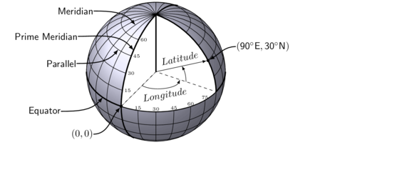
Traditionally locations were expressed as sets of latitudes and longitudes in degrees and minutes as this accounted for the earths curvature (assuming the Earth was a perfect sphere - which it is not). In the following graphic, a sphere representing Earth is partitioned into a series of vertical and horizontal rings at 15 degree increments around the center of the sphere.

The rings that run through the poles are called meridians and the prime meridian is the meridian from which the angle of all other meridians is compared and is therefore at a Longitude of $0^\circ$. The rings running perpendicular to the meridians are the parallels, the angles of which are measured relative to the equator (Latitude of $0^\circ$). Similarly the position of any point on the surface of the sphere can be expressed as its angles from the equator and prime meridian.

More recently, for smaller scale applications (for which the curvature is less relevant), it has been convenient to express locations as coordinates in meters as this lends itself well to simple calculations of distances between locations. In these situations the coordinates are only relevant within a particular reference region.

Similarly, different GPS devices and sources may store data in different projections. Hence it is important to be able to convert between different projections in order to combine geographical layers from different sources.

By way of example, I will take a shapefile of Magnetic Island with standard longlat projection and I will overlay the locations of a couple of koalas (UTM projection) recorded via a hand-held GPS as part of a radio tracking project.

#Orthographic coordinates
library(maps)
library(mapdata)
library(ggplot2)
map_data

function (map, region = ".", exact = FALSE, ...) 
{
    try_require("maps", "map_data")
    fortify(map(map, region, exact = exact, plot = FALSE, fill = TRUE, 
        ...))
}
<environment: namespace:ggplot2>

sessionInfo()

R version 3.3.2 (2016-10-31)
Platform: x86_64-pc-linux-gnu (64-bit)
Running under: BunsenLabs GNU/Linux 8.7 (Hydrogen)

locale:
 [1] LC_CTYPE=en_AU.UTF-8       LC_NUMERIC=C               LC_TIME=en_AU.UTF-8       
 [4] LC_COLLATE=en_AU.UTF-8     LC_MONETARY=en_AU.UTF-8    LC_MESSAGES=en_AU.UTF-8   
 [7] LC_PAPER=en_AU.UTF-8       LC_NAME=C                  LC_ADDRESS=C              
[10] LC_TELEPHONE=C             LC_MEASUREMENT=en_AU.UTF-8 LC_IDENTIFICATION=C       

attached base packages:
[1] stats     graphics  grDevices utils     datasets  methods   base     

other attached packages:
 [1] layers_1.2          PBSmapping_2.69.76  rgeos_0.3-22        rgdal_1.2-5        
 [5] ggmap_2.6.1         RgoogleMaps_1.4.1   mapping_0.1         oz_1.0-21          
 [9] maptools_0.9-2      shapefiles_0.7      foreign_0.8-61      GGally_1.3.0       
[13] reshape_0.8.6       scales_0.4.1        gridExtra_2.2.1     Cairo_1.5-9        
[17] knitcitations_1.0.7 coda_0.19-1         mvtnorm_1.0-5       bibtex_0.4.0       
[21] RefManageR_0.13.1   plyr_1.8.4          gdata_2.17.0        forcats_0.2.0      
[25] dplyr_0.5.0         purrr_0.2.2         readr_1.0.0         tidyr_0.6.1        
[29] tibble_1.2          ggplot2_2.2.1       tidyverse_1.1.1     xtable_1.8-2       
[33] sp_1.2-4            mapdata_2.2-6       maps_3.1.1          knitr_1.15.1       
[37] mgcv_1.8-17         nlme_3.1-131       

loaded via a namespace (and not attached):
 [1] httr_1.2.1         jsonlite_1.2       modelr_0.1.0       gtools_3.5.0       assertthat_0.1    
 [6] highr_0.6          lattice_0.20-29    digest_0.6.12      RColorBrewer_1.1-2 rvest_0.3.2       
[11] colorspace_1.3-2   Matrix_1.2-6       psych_1.6.12       XML_3.98-1.5       broom_0.4.2       
[16] haven_1.0.0        jpeg_0.1-8         lazyeval_0.2.0     proto_1.0.0        mnormt_1.5-5      
[21] RJSONIO_1.3-0      magrittr_1.5       readxl_0.1.1       evaluate_0.10      xml2_1.1.1        
[26] tools_3.3.2        hms_0.3            geosphere_1.5-5    stringr_1.2.0      munsell_0.4.3     
[31] grid_3.3.2         RCurl_1.95-4.8     rjson_0.2.15       bitops_1.0-6       codetools_0.2-9   
[36] gtable_0.2.0       DBI_0.5-1          reshape2_1.4.2     R6_2.2.0           lubridate_1.6.0   
[41] stringi_1.1.2      parallel_3.3.2     Rcpp_0.12.9        mapproj_1.2-4      png_0.1-7

world <- ggplot2:::map_data(map="worldHires")

Error: ggplot2 doesn't know how to deal with data of class list

 worldmap <- ggplot(world, aes(x=long, y=lat, group=group))+
  geom_path()+scale_y_continuous(breaks=c(-2:2 * 30))+scale_x_continuous(breaks=c(-4:4)*45)

Error in ggplot(world, aes(x = long, y = lat, group = group)): object 'world' not found

worldmap+coord_equal()

Error in eval(expr, envir, enclos): object 'worldmap' not found

worldmap+coord_map()

Error in eval(expr, envir, enclos): object 'worldmap' not found

worldmap+coord_map("ortho")

Error in eval(expr, envir, enclos): object 'worldmap' not found

worldmap+coord_map("cylindrical")

Error in eval(expr, envir, enclos): object 'worldmap' not found

worldmap+coord_map("guyou")

Error in eval(expr, envir, enclos): object 'worldmap' not found

#Convert dataframe into SpatialPointsDataFrame
#coordinates(df)=~long+lat

#Project latlong coordinates onto an ellipse
#proj4string(df)="+proj=longlat +ellps=WGS84 +datum=WGS84 +no_defs"
#+proj = the type of projection (lat/long)
#+ellps and +datum = the irregularity in the ellipse represented by planet earth

#Transform the projection into Euclidean distances
#project_df=spTransform(df, CRS("+proj=merc +zone=18s +ellps=WGS84 +datum=WGS84")) #projInfo(type="proj")

library(layers)
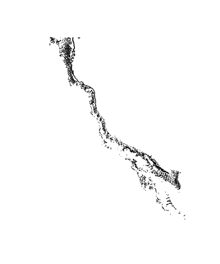
reefs <- reefs2SpatialPolygons(layers:::reefs)
#transform into utms
library(rgdal)
reefs.utm<-spTransform(reefs, CRSobj=CRS("+proj=utm +zone=55 +south +units=m +ellps=WGS84"))
plot(reefs.utm)

#or
library(maptools)
rf<-maptools:::.polylist2SpP(layers:::reefs)
proj4string(rf)<-"+proj=longlat +ellps=WGS84 +datum=WGS84 +no_defs"
rf.utm<-spTransform(rf, CRS("+proj=merc +zone=18s +ellps=WGS84 +datum=WGS84"))
plot(rf.utm)

Full mapping examples

Lets now bring many of these elements together to produce a couple of maps.

Site map

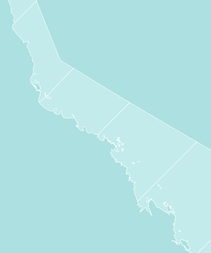
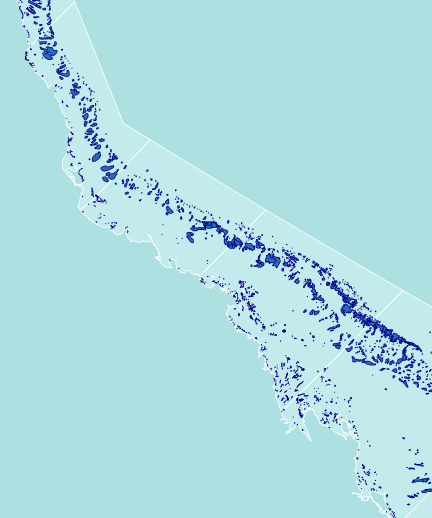
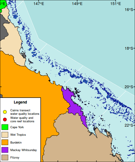
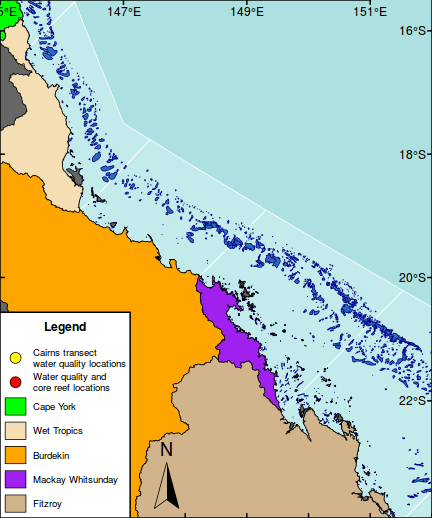
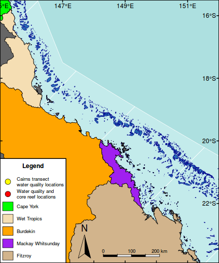
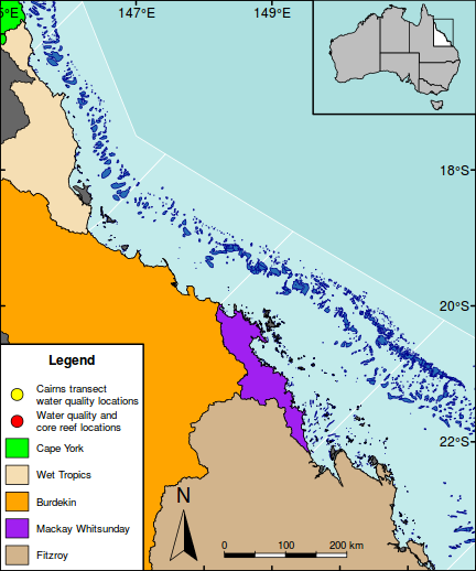
The following map is perhaps a little busy (not to mention a gaudy and kaleidoscopic), yet it functions to showcase the integration of a wide range of mapping features.

As an example of a reasonably complex map, it will involve many commands to build the up the figure. In such cases, it is easy to get rather lost and loose sight of the end goal. Hence, for inspiration and context I provide a glimpse of the final figure up front. Thereafter, the sequence of steps required to produce the figure (with progressive views of the figure) are available from the drop down.

Error in getinfo.shape(filen): Error opening SHP file

Error in lines(rivers.mp, col = "blue", lwd = 1): object 'rivers.mp' not found

Error in file(file, "rt"): cannot open the connection

Error in subset(sites, Sampling == "Reef"): object 'sites' not found

Error in subset(sites, Sampling == "Cairns"): object 'sites' not found

Show full code listing

library(rgeos)
library(maptools)
library(layers)
#Load and convert the base layers
reefs <- reefs2SpatialPolygons(layers:::reefs)
queensland <- reefs2SpatialPolygons(layers:::queensland)
nrm <- reefs2SpatialPolygons(layers:::nrm)
basin <- reefs2SpatialPolygons(layers:::basin)
basin.cy <- gUnaryUnion(basin[1:7], id=rep(1,7))  #unionSpatialPolygons(basin[1:7], IDs=rep(1,7))
basin.wt <- gUnaryUnion(basin[8:15], id=rep(1,8)) #unionSpatialPolygons(basin[8:15], IDs=rep(1,8))
basin.b <- gUnaryUnion(basin[16:20], id=rep(1,5))  #unionSpatialPolygons(basin[16:20], IDs=rep(1,5))
basin.mw <- gUnaryUnion(basin[21:24], id=rep(1,4)) #unionSpatialPolygons(basin[21:24], IDs=rep(1,4))
basin.f <- gUnaryUnion(basin[25:34], id=rep(1,10)) #unionSpatialPolygons(basin[25:34], IDs=rep(1,10))

#Set the device parameters and generate the blank base plot
opar<-par(mar=c(0,0,0,0), bg="#ADE0E0", xaxs="i",yaxs="i") #needs to be xaxs="i" otherwise axis extends 4%
plot(x=0, y=0,xlim=c(145.5,151.5), ylim=c(-23.9,-15.5), type="n", asp=1, axes=FALSE, ann=FALSE)

#Add the NRM region borders
plot(nrm, add=TRUE, col="#C3EBEB", border="white")

#Add the reefs
plot(reefs, add=TRUE, col="#276DB5", border="darkblue")

#Add the terrestrial shapes and color the different regions
plot(queensland, add=TRUE, col="grey40")

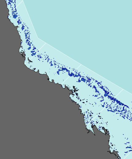
plot(basin.cy, add=TRUE,col="green")

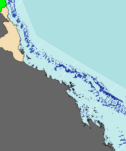
plot(basin.wt, add=TRUE, col="wheat")

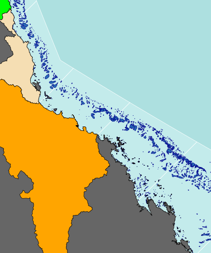
plot(basin.b, add=TRUE, col="orange")

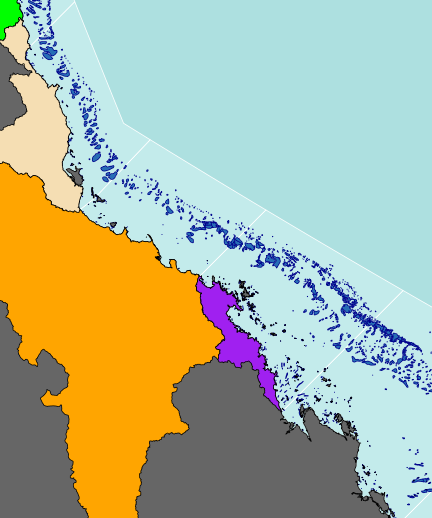
plot(basin.mw, add=TRUE, col="purple")

plot(basin.f, add=TRUE, col="tan")

#Add the axes with formatted degrees labels
axis(1, tck=0.01, lwd=2)

xs <- seq(145,152,b=2) #pretty(par()$usr[1:2])
axis(3, lwd=2,at=xs,lab=parse(text=degreeLabelsEW(xs)),tck=0.01, mgp=c(0,-1.3,0))

axis(2, las=1,tck=0.01,lwd=2)

ys <- pretty(par()$usr[3:4])
axis(4, las=1,tck=0.01,lwd=2,at=ys,lab=parse(text=degreeLabelsNS(ys)),tck=0.01, mgp=c(0,-2.3,0))

#Add the major rivers
rivers.mp <- readShapeLines("/home/murray/Work/Resources/GIS/rivers/MajorRivers")

Error in getinfo.shape(filen): Error opening SHP file

lines(rivers.mp, col="blue", lwd=1.0)

Error in lines(rivers.mp, col = "blue", lwd = 1): object 'rivers.mp' not found

#Add the major cities
#points(lat~long,data=layers:::towns12, pch=21, col="black", bg="white")
#text(lat~long,data=layers:::towns12, lab=town, col="white",pos=2)

sites <- read.csv("../downloads/data/GIS/sites.csv")

Error in file(file, "rt"): cannot open the connection

with(subset(sites,Sampling=="Reef"),points(LONGITUDE,LATITUDE,pch=21,col="black", bg="red"))

Error in subset(sites, Sampling == "Reef"): object 'sites' not found

with(subset(sites,Sampling=="Cairns"),points(LONGITUDE,LATITUDE,pch=21,col="black", bg="yellow"))

Error in subset(sites, Sampling == "Cairns"): object 'sites' not found

#Add a legend to the bottom left hand corner
maplegend("bottomleft",inset=0.0,cex=0.8,
       legend=c("Cairns transect\nwater quality locations",
         "Water quality and\ncore reef locations",
         "Cape York","Wet Tropics","Burdekin","Mackay Whitsunday","Fitzroy"),
       pch=c(21,21,NA,NA,NA,NA,NA),bty="o", box.lwd=2,
       bg="white",title="Legend",
       pt.bg=c("yellow","red",NA,NA,NA,NA,NA), col="black",
             fill=c(NA,NA,"green","wheat","orange","purple","tan"),
       border=c(NA,NA,1,1,1,1,1),pt.cex=2, #adj=c(1,0.5),
                y.intersp=1.5, x.intersp=2, title.font=2)

#Add a north arrow
north.arrow(147.7,-23,0.4, lab="N", lab.pos="above")

#Add scalebar
scalebar(c(148.3,-23.7),200,bg="tan",border=NA)

#Put a frame around the whole map
box(lwd=2)

#Add a context map in the top right corner
par(mar = c(0, 0, 0, 0), new = TRUE, fig = c(0.8*(1/1.216216), 1, 0.8, 1), xaxs="r",yaxs="r")
#A map of Austrlia
plot(oz2sp(oz),col="grey")

rect(145.5, -23.9,151.5,-15.5, lwd=1)

box(lwd=2)

#Highlight the GBR focal area
library(PBSmapping)
aa.ps <- SpatialPolygons2PolySet(oz2sp(oz))
# Clip 'PolySet' by given extent
aa.ps.clipped <- clipPolys(aa.ps, xlim = c(145.5,151.5), ylim = c(-23.9,-15.5))
# Convert clipped 'PolySet' back to SpatialPolygons
aa.1 <- PolySet2SpatialPolygons(aa.ps.clipped, close_polys=TRUE)
plot(aa.1, add=T, col="white")

Another site map with google background

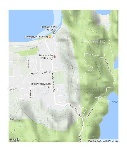
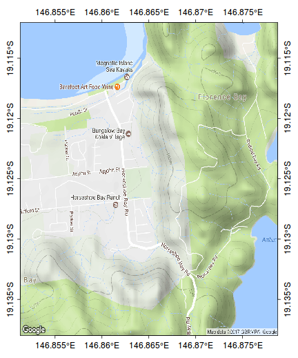
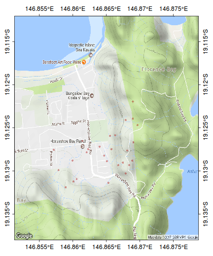
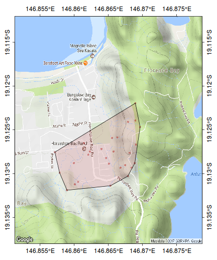
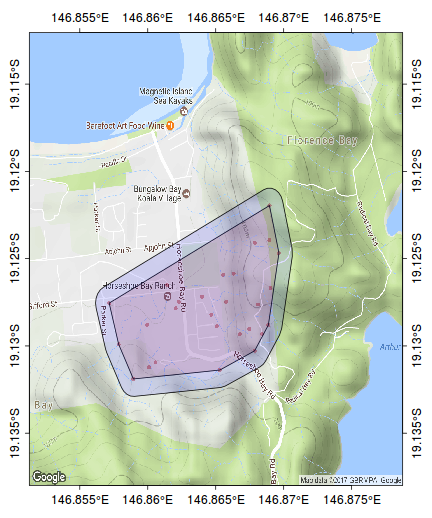
The following map represents the ranging behaviour of a koala over a 45 day period.

Error in file(file, "rt"): cannot open the connection

Show full code listing

par(mar=c(1,1,1,1))
library(ggmap)
terrain <- get_map(location=c(146.865,-19.125), zoom=15, maptype="terrain")
  bb <- as.numeric(attr(terrain,"bb"))
plot(bb[c(2,4)], bb[c(1,3)], type="n", axes=FALSE, ann=FALSE)

rasterImage(terrain, xleft=bb[2],ybottom=bb[1], xright=bb[4],ytop=bb[3], interpolate=FALSE)

xs <- pretty(bb[c(2,4)])
xs <- xs[c(-1,-length(xs))]

axis(1, pos=bb[1],at=xs, lab=parse(text=degreeLabelsEW(xs)), mgp=c(0,0.5,0),tck=-0.01)

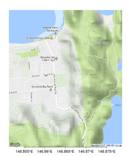
axis(3, pos=bb[3],at=xs, lab=parse(text=degreeLabelsEW(xs)), mgp=c(0,0.5,0),tck=-0.01)

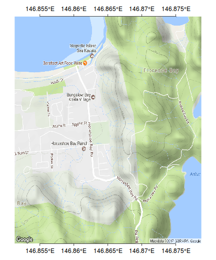
ys <- pretty(bb[c(1,3)])
ys <- ys[c(-1,-length(ys))]
axis(2, pos=bb[2],at=ys, lab=parse(text=degreeLabelsNS(ys)), mgp=c(0,0.5,0),tck=-0.01)

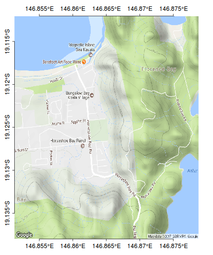
axis(4, pos=bb[4],at=ys, lab=parse(text=degreeLabelsNS(ys)), mgp=c(0,0.5,0),tck=-0.01)

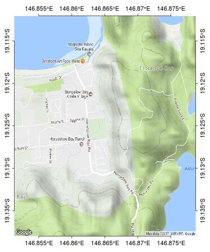
rect(bb[2],bb[1],bb[4],bb[3])

scalebar(c(146.79,-19.185),5)

north.arrow(146.8,-19.165,0.005)

kf45 <- read.csv(file="/home/murray/Dropbox/Work/Resources/Mapping/KF45.csv")

Error in file(file, "rt"): cannot open the connection

kf45.utm<-SpatialPointsDataFrame(kf45[,c(3,2)], data=kf45,proj4string=CRS("+proj=utm +zone=55 +south +ellps=WGS84"))
kf45.ll <- spTransform(kf45.utm, CRS("+proj=longlat +zone=55 +south +ellps=WGS84"))

plot(kf45.ll, add=T, col="#AA000060", pch=16, cex=0.75)

ch <- chull(sp:::coordinates(kf45.ll))
polygon(sp:::coordinates(kf45.ll[ch,]), col="#AA000020")

#make sure you close the ring
kf45.hull.sp<-SpatialPolygons(list(Polygons(list(Polygon(sp:::coordinates(kf45.ll[c(ch,ch[1]),]))), ID="kf45")))
library(rgeos)

plot(gBuffer(kf45.hull.sp, width=0.001), add=T, col="#0000FF20")

Spatial analyses

Calculating centroids

Centroids are the centers of polygons. Sometimes it can be useful to calculate the centroids of spatial polygons, particularly as a basis of data from which to calculate distances between spatial objects.

library(layers)
library(sp)
reefs <- reefs2SpatialPolygons(layers:::reefs)
library(rgeos)
reefs.c <- gCentroid(reefs)

Finding the nearest objects

Consider the situation where it is necessary to determine the distance to the nearest object. As an example, we may wish to calculate the distance of each reef from the mainland...

Step 1 - calculate the centroids of each reef (as above)

library(layers)
reefs <- reefs2SpatialPolygons(layers:::reefs)
library(rgeos)
reefs.c<-gCentroid(reefs, byid=TRUE)
reefs.df <- data.frame(reefs.c)

Step 2 - convert both the reefs and the mainland into UTM projections so that distances are represented in familiar units (m)

library(rgdal)
reefs.c.utm <- spTransform(reefs.c, CRS("+proj=utm +zone=55 +south +ellps=WGS84"))
queensland <- reefs2SpatialPolygons(layers:::queensland)
areas <- sapply(slot(queensland, "polygons"), slot, "area")
wch <- rev(order(areas))
mainland.sp <- SpatialPolygons(list(queensland@polygons[[wch[1]]]), proj4string=CRS('+proj=longlat'))
mainland.fort <- ggplot2:::fortify(mainland.sp)
mainland.utm <- spTransform(mainland.sp, CRS("+proj=utm +zone=55 +south +ellps=WGS84"))

## Quick plot to check conversions
plot(mainland.utm)
plot(reefs.c.utm, add=TRUE)

Step 3 - calculate the distance in meters from each reef to each point of the mainland Queensland polygon

dis <- gDistance(reefs.c.utm, mainland.utm, byid=TRUE)

Error in RGEOSDistanceFunc(spgeom1, spgeom2, byid, "rgeos_distance"): object 'mainland.utm' not found

min.dis<-apply(dis,2,min)

Error in apply(dis, 2, min): object 'dis' not found

Step 3 - calculate the distance in meters from each reef to each point of the mainland Queensland polygon

n<-apply(dis,2,function(x) {
  m<-min(x)
  n <- which(x==m)
  n
})

Error in apply(dis, 2, function(x) {: object 'dis' not found

reefs.df$mainlandLONGITUDE <- mainland.fort[n,'long']

Error in eval(expr, envir, enclos): object 'mainland.fort' not found

reefs.df$mainlandLATITUDE <- mainland.fort[n,'lat']

Error in eval(expr, envir, enclos): object 'mainland.fort' not found

reefs.df$Distance <- min.dis

Error in eval(expr, envir, enclos): object 'min.dis' not found

head(reefs.df)

              x         y
reef 1 144.4248 -10.39163
reef 2 142.0543 -10.35641
reef 3 142.1080 -10.35225
reef 4 143.9400 -10.35258
reef 5 142.1081 -10.34994
reef 6 142.1201 -10.37453

#pt <- data.frame(X=c(144.4,143.9),Y=c(-10.3,-10.35))
##eucidean distance between points (in the units of the supplied X and Y)
#nearestReef<-function (pts, pt) 
#{
#    pts$Xorig <- pt$X
#    pts$Yorig <- pt$Y
#    pts$dist <- sqrt(pts$Xorig - pts$X)^2 + (pts$Yorig - pts$Y)^2
#    return(dist=list(min(pts$dist),reef=pts$dist == min(pts$dist)))
#}
#
#library(plyr)
#pt<-adply(pt,1,function(x){
#  nr <- nearestReef(reefs.c, x)
#  data.frame(Dist=nr[[1]], Reef=reefs.c[nr[[2]],])
#})
#head(pt)
#
#findDistances(pt,neighbours=reefs.c)
#
#
##or if need nearest envelope
#reefs.b<-gEnvelope(reefs, byid=TRUE)
#library(ggplot2)
#reefs.b<-fortify(reefs.b)
#nms <- colnames(reefs.b)
#colnames(reefs.b)[1:2] <- c("X","Y")
#reefs.b <- reefs.b[,1:2]
#findDistances(pt,neighbours=reefs.b)

Tutorial 5.4 - Mapping and spatial analyses in R

Spatial data classes

Spatial packages

Obtaining spatial data

maps and mapdata packages - world maps

ESRI Shapefiles

Working exclusively with the shp file

Converting a shp into a simple data frame

Reading shp directly into a spatial class

Reading shapefiles into a SpatialPolygonsDataFrame

Other regionally specific packages - e.g. oz

mapping - my (recycled from Glenn De'ath) map layers

Queensland

gbr

basin

whagbr

bioregion

zoning

nrm

Raster images - map backgrounds

ggmap

Adornments

Scale bar

North arrow

Degrees labels

Map legends

Reprojections

Full mapping examples

Site map

Another site map with google background

Spatial analyses

Calculating centroids

Finding the nearest objects

Welcome to the end of this tutorial

`maps` and `mapdata` packages - world maps

Other regionally specific packages - e.g. `oz`

`mapping` - my (recycled from Glenn De'ath) map layers