Workshop 9.15.3a: Mixed effects models
Murray Logan
22-09-2014
Linear models
\[
\begin{align*}
y_{i} &= \beta_0 + \beta_1 \times x_{i} + \varepsilon_i\\
\epsilon_i&\sim\mathcal{N}(0, \sigma^2) \\
\end{align*}
\]
Linear models
Linear models
Linear models
how maximize power?
increase replication
add covariates (if noise predictable)
Linear models
how maximize power?
increase replication
add covariates (if noise predictable)
block
Linear modelling assumptions
\[
\begin{align*}
y_{i} &= \beta_0 + \beta_1 \times x_{i} + \varepsilon_i\\
\epsilon_i&\sim\mathcal{N}(0, \sigma^2) \\
\end{align*}
\]
Non-independence
one response is triggered by another
temporal/spatial autocorrelation
nested (hierarchical) design structures
Hierarchical models
linear model with separate covariance structure per block
fixed and random factors (effects)
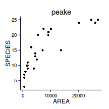
Example
data.rcb <- read.csv ('../data/data.rcb.csv' )
head (data.rcb) y x block
1 281.1 18.59 Block1
2 295.7 26.05 Block1
3 328.3 40.10 Block1
4 360.2 63.57 Block1
5 276.7 14.12 Block1
6 349.0 62.89 Block1library (car)
scatterplot (y~x, data.rcb)
Example
ggplot (data.rcb, aes (y= y, x= x,color= block))+geom_point ()+
geom_smooth (method= 'lm' )Error: could not find function "ggplot"
Example
Simple linear regression - wrong
data.rcb.lm <- lm (y~x, data.rcb)
library (nlme)
data.rcb.gls <- gls (y~x, data.rcb, method= 'REML' )
Example
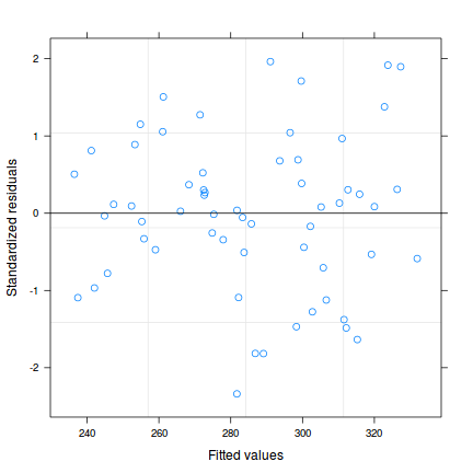
Model validation
plot (data.rcb.gls)
Example
plot (residuals (data.rcb.gls, type= 'normalized' ) ~
data.rcb$block)
Example
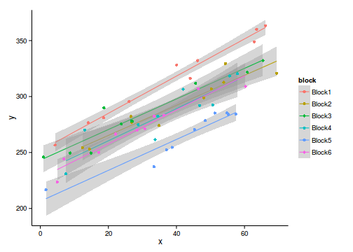
library (ggplot2)
ggplot (data.rcb, aes (y= y, x= x, color= block))+
geom_smooth (method= "lm" )+geom_point ()+theme_classic ()
ggplot (data.rcb, aes (y= y, x= x))+
geom_smooth (method= "lm" )+geom_point ()+theme_classic ()
Example
library (nlme)
data.rcb.gls1 <- gls (y~x+block, data.rcb, method= 'REML' )
plot (data.rcb.gls)
Example
plot (residuals (data.rcb.gls1, type= 'normalized' ) ~
data.rcb$block)
Example
Looks good, but for INDEPENDENCE
Can we deal with that with correlation structure ?
Example
library (nlme)
data.rcb.gls2<-gls (y~x,data.rcb,
correlation= corCompSymm (form= ~1 |block),
method= "REML" )
plot (residuals (data.rcb.gls2, type= 'normalized' ) ~
fitted (data.rcb.gls2))
Example
plot (residuals (data.rcb.gls2, type= 'normalized' ) ~
data.rcb$block)
Example
summary (data.rcb.gls2)Generalized least squares fit by REML
Model: y ~ x
Data: data.rcb
AIC BIC logLik
459 467.2 -225.5
Correlation Structure: Compound symmetry
Formula: ~1 | block
Parameter estimate(s):
Rho
0.8053
Coefficients:
Value Std.Error t-value p-value
(Intercept) 232.82 7.823 29.76 0
x 1.46 0.064 22.87 0
Correlation:
(Intr)
x -0.292
Standardized residuals:
Min Q1 Med Q3 Max
-2.19175 -0.59481 0.05261 0.59571 1.83322
Residual standard error: 20.18
Degrees of freedom: 60 total; 58 residual
Linear mixed effects model
data.rcb.lm <- lm (y~x, data.rcb)
plot (rstandard (data.rcb.lm) ~ fitted (data.rcb.lm))
plot (rstandard (data.rcb.lm) ~ data.rcb$block)
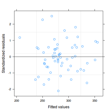
data.rcb.lme <- lme (y~x, random= ~1 |block, data.rcb,
method= 'REML' )
plot (data.rcb.lme)
plot (residuals (data.rcb.lme, type= 'normalized' ) ~ fitted (data.rcb.lme))
plot (residuals (data.rcb.lme, type= 'normalized' ) ~ data.rcb$block)
Linear mixed effects model
summary (data.rcb.lme)Linear mixed-effects model fit by REML
Data: data.rcb
AIC BIC logLik
459 467.2 -225.5
Random effects:
Formula: ~1 | block
(Intercept) Residual
StdDev: 18.11 8.905
Fixed effects: y ~ x
Value Std.Error DF t-value p-value
(Intercept) 232.82 7.823 53 29.76 0
x 1.46 0.064 53 22.87 0
Correlation:
(Intr)
x -0.292
Standardized Within-Group Residuals:
Min Q1 Med Q3 Max
-2.09947 -0.57994 -0.04874 0.56685 2.49464
Number of Observations: 60
Number of Groups: 6
Linear mixed effects model
anova (data.rcb.lme) numDF denDF F-value p-value
(Intercept) 1 53 1452.3 <.0001
x 1 53 523.2 <.0001intervals (data.rcb.lme)Approximate 95% confidence intervals
Fixed effects:
lower est. upper
(Intercept) 217.128 232.819 248.511
x 1.331 1.459 1.587
attr(,"label")
[1] "Fixed effects:"
Random Effects:
Level: block
lower est. upper
sd((Intercept)) 9.598 18.11 34.17
Within-group standard error:
lower est. upper
7.362 8.905 10.773
Linear mixed effects model
vc<-as.numeric (as.matrix (VarCorr (data.rcb.lme))[,1 ])
vc/sum (vc)[1] 0.8052 0.1948
Linear mixed effects model
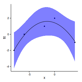
library (effects)
plot (allEffects (data.rcb.lme))
Linear mixed effects model
predict (data.rcb.lme, newdata= data.frame (x= 30 :40 ),level= 0 ) [1] 276.6 278.1 279.5 281.0 282.4 283.9 285.3
[8] 286.8 288.3 289.7 291.2
attr(,"label")
[1] "Predicted values"
Linear mixed effects model
predict (data.rcb.lme, newdata= data.frame (x= 30 :40 ,
block= 'Block1' ),level= 1 )Block1 Block1 Block1 Block1 Block1 Block1 Block1
302.7 304.2 305.7 307.1 308.6 310.0 311.5
Block1 Block1 Block1 Block1
313.0 314.4 315.9 317.3
attr(,"label")
[1] "Predicted values"
Linear mixed effects model
Step 1. gather model coefficients
coefs <- fixef (data.rcb.lme)
coefs(Intercept) x
232.819 1.459
Linear mixed effects model
Step 2. generate prediction model matrix
xs <- seq (min (data.rcb$x), max (data.rcb$x), l= 100 )
Xmat <- model.matrix (~x, data.frame (x= xs))
head (Xmat) (Intercept) x
1 1 0.9373
2 1 1.6292
3 1 2.3211
4 1 3.0130
5 1 3.7048
6 1 4.3967
Linear mixed effects model
Step 3. calculate predicted y
ys <- t (coefs %*% t (Xmat))
head (ys) [,1]
1 234.2
2 235.2
3 236.2
4 237.2
5 238.2
6 239.2
Linear mixed effects model
Step 3. calculate confidence interval
SE <- sqrt (diag (Xmat %*% vcov (data.rcb.lme) %*% t (Xmat)))
CI <- 2 *SE
#OR
CI <- qt (0.975 ,length (data.rcb$x)-2 )*SE
data.rcb.pred <- data.frame (x= xs, fit= ys, se= SE,
lower= ys-CI, upper= ys+CI)
head (data.rcb.pred) x fit se lower upper
1 0.9373 234.2 7.806 218.6 249.8
2 1.6292 235.2 7.794 219.6 250.8
3 2.3211 236.2 7.781 220.6 251.8
4 3.0130 237.2 7.769 221.7 252.8
5 3.7048 238.2 7.758 222.7 253.8
6 4.3967 239.2 7.746 223.7 254.7
Linear mixed effects model
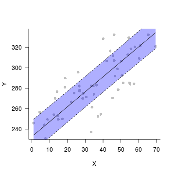
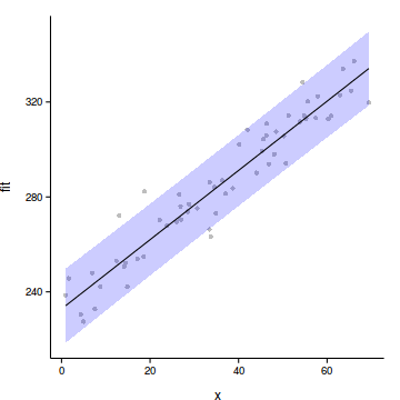
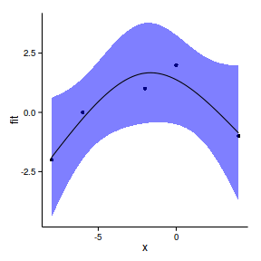
Step 4. plot it
plot (fit~x, data= data.rcb.pred,type= 'n' ,axes= F, ann= F)
points (y~x, data= data.rcb, pch= 16 , col= 'grey' )
with (data.rcb.pred, polygon (c (x,rev (x)), c (lower, rev (upper)),
col= "#0000FF50" ,border= FALSE ))
lines (fit~x,data= data.rcb.pred)
lines (lower~x,data= data.rcb.pred, lty= 2 )
lines (upper~x,data= data.rcb.pred, lty= 2 )
axis (1 )
mtext ('X' ,1 ,line= 3 )
axis (2 ,las= 1 )
mtext ('Y' ,2 ,line= 3 )
box (bty= 'l' )
Linear mixed effects model
Linear mixed effects model
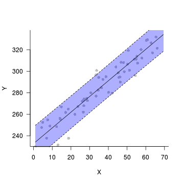
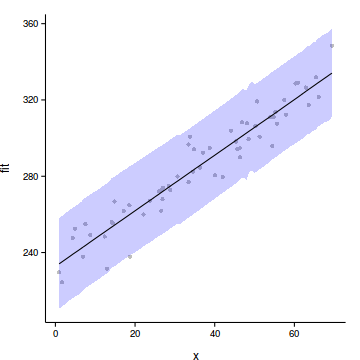
Step 4. plot it
data.rcb$res <- predict (data.rcb.lme, level= 0 )-
residuals (data.rcb.lme)
plot (fit~x, data= data.rcb.pred,type= 'n' ,axes= F, ann= F)
points (res~x, data= data.rcb, pch= 16 , col= 'grey' )
with (data.rcb.pred, polygon (c (x,rev (x)), c (lower, rev (upper)),
col= "#0000FF50" ,border= FALSE ))
lines (fit~x,data= data.rcb.pred)
lines (lower~x,data= data.rcb.pred, lty= 2 )
lines (upper~x,data= data.rcb.pred, lty= 2 )
axis (1 )
mtext ('X' ,1 ,line= 3 )
axis (2 ,las= 1 )
mtext ('Y' ,2 ,line= 3 )
box (bty= 'l' )
Linear mixed effects model
Linear mixed effects model
library (ggplot2)
data.rcb$res <- predict (data.rcb.lme, level= 0 )+
residuals (data.rcb.lme)
ggplot (data.rcb.pred, aes (y= fit, x= x))+
geom_point (data= data.rcb, aes (y= res), col= 'grey' )+
geom_ribbon (aes (ymin= lower, ymax= upper),
fill= 'blue' , alpha= 0.2 )+
geom_line ()+
theme_classic ()+
theme (axis.title.y= element_text (vjust= 2 ),
axis.title.x= element_text (vjust= -1 ))
Linear mixed effects model
Bayesian HMM
modelString = '
model{
for (i in 1:n) {
y[i] ~ dnorm(mu[i], tau)
mu[i] <- beta.blk[block[i]] + alpha + beta*x[i]
}
alpha ~ dnorm(0,1.0E-06)
beta ~ dnorm(0,1.0E-06)
for (i in 1:nBlock) {
beta.blk[i] ~ dnorm(0, tau.blk)
}
tau <- 1/(sigma * sigma)
tau.blk <- 1/(sigma.blk * sigma.blk)
sigma ~ dunif(0,1000)
sigma.blk ~ dunif(0,1000)
}
'
writeLines (modelString, con= 'HMM.jags' )
library (R2jags)
data.list <- with (data.rcb, list (y= y, x= x,
block= as.numeric (block),
n= nrow (data.rcb),
nBlock= length (unique (block))
))
data.rcb.jags <- jags (data= data.list, inits= NULL ,
param = c ('alpha' ,'beta' ,'beta.blk' ,'sigma' ,'sigma.blk' ),
model.file = 'HMM.jags' ,
n.chains= 3 , n.iter= 20000 , n.burnin = 10000 ,
n.thin= 10 )Compiling model graph
Resolving undeclared variables
Allocating nodes
Graph Size: 320
Initializing modelprint (data.rcb.jags)Inference for Bugs model at "HMM.jags", fit using jags,
3 chains, each with 20000 iterations (first 10000 discarded), n.thin = 10
n.sims = 3000 iterations saved
mu.vect sd.vect 2.5% 25%
alpha 233.017 12.408 208.482 226.390
beta 1.460 0.066 1.331 1.416
beta.blk[1] 26.029 12.470 0.851 19.397
beta.blk[2] 0.822 12.415 -24.059 -5.842
beta.blk[3] 7.276 12.461 -17.742 0.613
beta.blk[4] -2.076 12.419 -26.452 -8.752
beta.blk[5] -29.259 12.346 -55.191 -35.653
beta.blk[6] -3.979 12.413 -28.779 -10.533
sigma 9.139 0.905 7.601 8.495
sigma.blk 26.062 14.997 12.056 17.570
deviance 434.129 4.324 427.692 430.899
50% 75% 97.5% Rhat n.eff
alpha 233.062 239.456 257.772 1.002 3000
beta 1.460 1.505 1.586 1.001 2400
beta.blk[1] 26.023 32.627 51.147 1.003 1900
beta.blk[2] 0.916 7.619 25.225 1.003 2700
beta.blk[3] 7.336 14.138 30.461 1.003 1900
beta.blk[4] -1.995 4.644 22.392 1.004 3000
beta.blk[5] -29.161 -22.484 -5.543 1.004 3000
beta.blk[6] -3.801 2.796 19.772 1.003 1800
sigma 9.076 9.708 11.055 1.002 1800
sigma.blk 22.466 29.756 62.270 1.002 3000
deviance 433.502 436.588 444.495 1.001 3000
For each parameter, n.eff is a crude measure of effective sample size,
and Rhat is the potential scale reduction factor (at convergence, Rhat=1).
DIC info (using the rule, pD = var(deviance)/2)
pD = 9.4 and DIC = 443.5
DIC is an estimate of expected predictive error (lower deviance is better).
Bayesian HMM
modelString = '
model{
for (i in 1:n) {
y[i] ~ dnorm(mu[i], tau)
mu[i] <- beta.blk[block[i]] + alpha + beta*x[i]
res[i] <- y[i]-mu[i]
}
alpha ~ dnorm(0,1.0E-06)
beta ~ dnorm(0,1.0E-06)
for (i in 1:nBlock) {
beta.blk[i] ~ dnorm(0, tau.blk)
}
tau <- 1/(sigma * sigma)
tau.blk <- 1/(sigma.blk * sigma.blk)
sigma ~ dunif(0,1000)
sigma.blk ~ dunif(0,1000)
sd.res <- sd(res[])
sd.x <-abs(beta)*sd(x[])
sd.blk <- sd(beta.blk[])
}
'
writeLines (modelString, con= 'HMM1.jags' )
library (R2jags)
data.list <- with (data.rcb, list (y= y, x= x,
block= as.numeric (block),
n= nrow (data.rcb),
nBlock= length (unique (block))
))
data.rcb.jags <- jags (data= data.list, inits= NULL ,
param = c ('alpha' ,'beta' ,'beta.blk' ,'sigma' ,'sigma.blk' ,'sd.res' ,'sd.x' ,'sd.blk' ,'res' ),
model.file = 'HMM1.jags' ,
n.chains= 3 , n.iter= 20000 , n.burnin = 10000 ,
n.thin= 10 )Compiling model graph
Resolving undeclared variables
Allocating nodes
Graph Size: 388
Initializing modelprint (data.rcb.jags)Inference for Bugs model at "HMM1.jags", fit using jags,
3 chains, each with 20000 iterations (first 10000 discarded), n.thin = 10
n.sims = 3000 iterations saved
mu.vect sd.vect 2.5% 25%
alpha 232.468 11.955 207.386 225.958
beta 1.462 0.065 1.332 1.418
beta.blk[1] 26.538 11.951 4.472 19.772
beta.blk[2] 1.167 11.840 -21.593 -5.557
beta.blk[3] 7.805 11.909 -14.929 1.236
beta.blk[4] -1.521 11.835 -24.031 -8.017
beta.blk[5] -28.825 11.930 -52.010 -35.631
beta.blk[6] -3.508 11.868 -25.906 -10.339
res[1] -5.069 3.230 -11.486 -7.206
res[2] -1.436 3.059 -7.546 -3.420
res[3] 10.692 2.936 4.874 8.776
res[4] 8.215 3.342 1.452 6.037
res[5] -2.941 3.363 -9.640 -5.167
res[6] -1.976 3.320 -8.686 -4.151
res[7] 7.650 3.425 0.669 5.434
res[8] 5.492 2.971 -0.393 3.587
res[9] -7.047 2.952 -12.871 -8.970
res[10] -8.743 3.718 -16.092 -11.160
res[11] -1.497 3.314 -7.903 -3.761
res[12] 2.464 3.379 -4.091 0.165
res[13] -4.987 2.991 -10.778 -7.011
res[14] 4.142 3.016 -1.789 2.085
res[15] 0.338 3.095 -5.641 -1.753
res[16] -10.488 2.930 -16.189 -12.441
res[17] -0.371 3.024 -6.188 -2.411
res[18] -14.346 3.563 -21.224 -16.720
res[19] 9.650 3.020 3.703 7.578
res[20] 16.181 3.107 10.133 14.098
res[21] -3.706 3.778 -10.998 -6.384
res[22] -12.397 3.068 -18.211 -14.387
res[23] 4.911 3.123 -1.164 2.850
res[24] -3.536 3.210 -9.683 -5.653
res[25] 22.207 3.001 16.521 20.233
res[26] -1.885 2.928 -7.556 -3.806
res[27] 4.413 3.453 -2.272 2.160
res[28] -1.222 2.929 -6.895 -3.133
res[29] -7.639 3.597 -14.517 -10.155
res[30] 0.274 2.945 -5.442 -1.667
res[31] -18.790 2.939 -24.512 -20.720
res[32] 14.227 2.931 8.490 12.317
res[33] 0.822 2.934 -4.921 -1.113
res[34] 20.198 3.365 13.723 17.982
res[35] 4.933 3.187 -1.476 2.798
res[36] -7.344 2.973 -13.255 -9.298
res[37] 6.197 3.130 -0.068 4.102
res[38] -11.077 3.556 -17.979 -13.447
res[39] -12.634 3.029 -18.744 -14.619
res[40] 1.985 2.991 -3.821 0.031
res[41] -3.433 3.131 -9.645 -5.478
res[42] 0.548 2.955 -5.219 -1.418
res[43] 1.642 3.076 -4.371 -0.340
res[44] -5.608 2.946 -11.335 -7.602
res[45] -5.462 2.954 -11.192 -7.423
res[46] -0.436 3.084 -6.492 -2.432
res[47] 10.659 3.917 2.920 7.978
res[48] -15.150 2.985 -20.943 -17.110
res[49] 6.703 3.016 0.772 4.772
res[50] 3.988 2.982 -1.918 2.044
res[51] 4.641 2.877 -0.992 2.737
res[52] -8.011 3.481 -14.854 -10.333
res[53] -2.395 2.869 -7.988 -4.292
res[54] -3.938 2.994 -9.864 -5.840
res[55] -12.497 3.311 -18.846 -14.683
res[56] 5.083 3.247 -1.227 2.966
res[57] 5.185 2.917 -0.581 3.313
res[58] 1.121 2.897 -4.500 -0.804
res[59] 10.369 3.058 4.320 8.288
res[60] -0.593 2.871 -6.207 -2.482
sd.blk 18.143 1.323 15.547 17.242
sd.res 8.938 0.303 8.541 8.715
sd.x 27.595 1.236 25.142 26.772
sigma 9.137 0.925 7.559 8.483
sigma.blk 25.505 13.189 12.020 17.461
deviance 434.157 4.532 427.636 430.749
50% 75% 97.5% Rhat n.eff
alpha 232.724 239.276 255.475 1.001 3000
beta 1.462 1.507 1.587 1.001 3000
beta.blk[1] 26.141 32.993 51.875 1.001 3000
beta.blk[2] 1.027 7.692 25.605 1.001 3000
beta.blk[3] 7.583 14.295 32.632 1.001 3000
beta.blk[4] -1.678 4.896 22.754 1.002 3000
beta.blk[5] -29.028 -22.177 -3.990 1.001 3000
beta.blk[6] -3.489 3.016 20.591 1.002 3000
res[1] -4.930 -2.870 1.052 1.001 3000
res[2] -1.346 0.681 4.299 1.001 3000
res[3] 10.713 12.706 16.390 1.001 3000
res[4] 8.199 10.371 14.888 1.001 3000
res[5] -2.799 -0.674 3.426 1.001 2900
res[6] -1.990 0.167 4.630 1.001 3000
res[7] 7.643 9.864 14.420 1.001 3000
res[8] 5.499 7.470 11.189 1.001 3000
res[9] -7.045 -5.055 -1.437 1.001 3000
res[10] -8.579 -6.277 -1.495 1.001 2900
res[11] -1.575 0.708 5.352 1.001 2300
res[12] 2.393 4.735 9.359 1.001 2500
res[13] -5.008 -3.056 1.027 1.002 1100
res[14] 4.048 6.175 10.178 1.002 1500
res[15] 0.294 2.346 6.608 1.002 1000
res[16] -10.542 -8.577 -4.701 1.002 1300
res[17] -0.389 1.586 5.720 1.002 1000
res[18] -14.394 -12.025 -7.313 1.002 1100
res[19] 9.566 11.684 15.690 1.002 1600
res[20] 16.124 18.199 22.478 1.004 980
res[21] -3.697 -1.195 3.666 1.001 3000
res[22] -12.432 -10.396 -6.170 1.001 3000
res[23] 4.882 7.001 11.208 1.001 3000
res[24] -3.627 -1.430 2.911 1.001 2900
res[25] 22.167 24.164 28.292 1.001 3000
res[26] -1.904 0.046 4.021 1.001 3000
res[27] 4.352 6.673 11.173 1.001 2700
res[28] -1.237 0.701 4.691 1.001 3000
res[29] -7.639 -5.241 -0.691 1.001 3000
res[30] 0.241 2.178 6.136 1.001 3000
res[31] -18.813 -16.841 -13.029 1.003 3000
res[32] 14.224 16.227 19.808 1.006 3000
res[33] 0.792 2.773 6.531 1.003 3000
res[34] 20.176 22.420 26.901 1.003 2900
res[35] 4.909 7.106 11.221 1.001 3000
res[36] -7.349 -5.340 -1.645 1.002 3000
res[37] 6.185 8.333 12.381 1.001 3000
res[38] -11.134 -8.688 -3.957 1.001 3000
res[39] -12.649 -10.575 -6.714 1.002 3000
res[40] 1.953 3.979 7.877 1.002 3000
res[41] -3.489 -1.459 2.898 1.001 3000
res[42] 0.523 2.444 6.654 1.001 3000
res[43] 1.599 3.565 7.879 1.001 3000
res[44] -5.657 -3.696 0.374 1.001 3000
res[45] -5.507 -3.561 0.405 1.001 3000
res[46] -0.486 1.493 5.842 1.001 3000
res[47] 10.655 13.305 18.190 1.001 3000
res[48] -15.163 -13.226 -9.216 1.001 3000
res[49] 6.670 8.624 12.799 1.001 3000
res[50] 3.945 5.908 10.114 1.001 3000
res[51] 4.616 6.583 10.265 1.006 340
res[52] -8.021 -5.633 -1.069 1.006 380
res[53] -2.420 -0.436 3.125 1.006 350
res[54] -4.013 -1.952 1.880 1.005 450
res[55] -12.558 -10.298 -6.036 1.004 640
res[56] 5.029 7.235 11.472 1.004 600
res[57] 5.108 7.143 10.842 1.005 400
res[58] 1.083 3.069 6.854 1.006 340
res[59] 10.361 12.394 16.464 1.006 420
res[60] -0.659 1.364 4.970 1.006 360
sd.blk 18.151 19.019 20.733 1.001 2100
sd.res 8.876 9.095 9.697 1.002 3000
sd.x 27.600 28.443 29.948 1.001 3000
sigma 9.048 9.699 11.141 1.001 3000
sigma.blk 22.226 29.264 61.728 1.001 3000
deviance 433.308 436.654 444.924 1.001 3000
For each parameter, n.eff is a crude measure of effective sample size,
and Rhat is the potential scale reduction factor (at convergence, Rhat=1).
DIC info (using the rule, pD = var(deviance)/2)
pD = 10.3 and DIC = 444.4
DIC is an estimate of expected predictive error (lower deviance is better).
Bayesian HMM
coefs <- data.rcb.jags$BUGSoutput$sims.matrix[,c ('alpha' ,'beta' )]
xs <- seq (min (data.rcb$x), max (data.rcb$x), l= 100 )
Xmat <- model.matrix (~x, data.frame (x= xs))
head (Xmat) (Intercept) x
1 1 0.9373
2 1 1.6292
3 1 2.3211
4 1 3.0130
5 1 3.7048
6 1 4.3967pred <- coefs %*% t (Xmat)
library (plyr)
library (coda)
data.rcb.pred <- adply (pred,2 ,function(x) {
data.frame (fit= median (x),HPDinterval (as.mcmc (x)))
})
data.rcb.pred <- cbind (x= xs,data.rcb.pred)
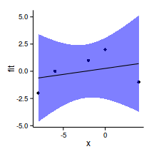
ggplot (data.rcb.pred, aes (y= fit, x= x))+
# geom_point(data=data.rcb, aes(y=res), col='grey')+
geom_ribbon (aes (ymin= lower, ymax= upper),
fill= 'blue' , alpha= 0.2 )+
geom_line ()+
theme_classic ()+
theme (axis.title.y= element_text (vjust= 2 ),
axis.title.x= element_text (vjust= -1 ))
Xmat <- model.matrix (~x, data= data.rcb)
pred <- coefs %*% t (Xmat)
library (plyr)
library (coda)
res <- adply (
data.rcb.jags$BUGSoutput$sims.matrix[,10 :69 ],
2 ,function(x) {
data.frame (res= median (x))})$res
res <- adply (pred,2 ,function(x) {data.frame (fit= median (x))})$fit - res
data.rcb$res1 <- res
ggplot (data.rcb.pred, aes (y= fit, x= x))+
geom_point (data= data.rcb, aes (y= res1), col= 'grey' )+
geom_ribbon (aes (ymin= lower, ymax= upper),
fill= 'blue' , alpha= 0.2 )+
geom_line ()+
theme_classic ()+
theme (axis.title.y= element_text (vjust= 2 ),
axis.title.x= element_text (vjust= -1 ))
Nested design
data.nest <- read.csv ('../data/data.nest.csv' )
head (data.nest) y Region Sites Quads
1 32.26 A S1 1
2 32.40 A S1 2
3 37.20 A S1 3
4 36.59 A S1 4
5 35.45 A S1 5
6 37.08 A S1 6
Nested design
library (ggplot2)
data.nest$Sites <- factor (data.nest$Sites, levels= paste0 ('S' ,1 :nSites))
ggplot (data.nest, aes (y= y, x= 1 ,color= Region)) + geom_boxplot () +
facet_grid (.~Sites) +
scale_x_continuous ('' , breaks= NULL )+theme_classic ()
Nested design
#Effects of treatment
library (plyr)
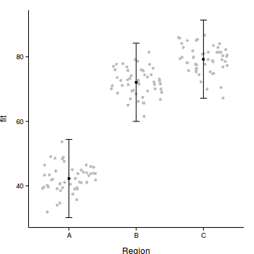
boxplot (y~Region, ddply (data.nest, ~Region+Sites,
numcolwise (mean, na.rm= T)))
Nested design
#Site effects
boxplot (y~Sites, ddply (data.nest, ~Region+Sites+Quads,
numcolwise (mean, na.rm= T)))
Nested design
library (nlme)
data.nest.lme <- lme (y~Region, random= ~1 |Sites, data.nest)
plot (data.nest.lme)
Nested design
plot (data.nest$Region, residuals (data.nest.lme,
type= 'normalized' ))
Nested design
summary (data.nest.lme)Linear mixed-effects model fit by REML
Data: data.nest
AIC BIC logLik
927.7 942.7 -458.9
Random effects:
Formula: ~1 | Sites
(Intercept) Residual
StdDev: 13.66 4.372
Fixed effects: y ~ Region
Value Std.Error DF t-value p-value
(Intercept) 42.28 6.139 135 6.887 0.0000
RegionB 29.85 8.682 12 3.438 0.0049
RegionC 37.02 8.682 12 4.264 0.0011
Correlation:
(Intr) ReginB
RegionB -0.707
RegionC -0.707 0.500
Standardized Within-Group Residuals:
Min Q1 Med Q3 Max
-2.603787 -0.572952 0.004954 0.620915 2.765602
Number of Observations: 150
Number of Groups: 15
Nested design
VarCorr (data.nest.lme)Sites = pdLogChol(1)
Variance StdDev
(Intercept) 186.55 13.658
Residual 19.12 4.372anova (data.nest.lme) numDF denDF F-value p-value
(Intercept) 1 135 331.8 <.0001
Region 2 12 10.2 0.0026
Nested design
library (multcomp)
summary (glht (data.nest.lme, linfct= mcp (Region= "Tukey" )))
     Simultaneous Tests for General Linear Hypotheses

Multiple Comparisons of Means: Tukey Contrasts


Fit: lme.formula(fixed = y ~ Region, data = data.nest, random = ~1 |
    Sites)

Linear Hypotheses:
           Estimate Std. Error z value Pr(>|z|)
B - A == 0    29.85       8.68    3.44   0.0017
C - A == 0    37.02       8.68    4.26   <0.001
C - B == 0     7.17       8.68    0.83   0.6867

B - A == 0 **
C - A == 0 ***
C - B == 0
---
Signif. codes:
0 '***' 0.001 '**' 0.01 '*' 0.05 '.' 0.1 ' ' 1
(Adjusted p values reported -- single-step method)
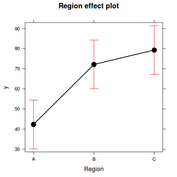
Nested design
library (effects)
plot (allEffects (data.nest.lme))
Linear mixed effects model
Step 1. gather model coefficients and model matrix
coefs <- fixef (data.nest.lme)
coefs(Intercept) RegionB RegionC
42.28 29.85 37.02 xs <- levels (data.nest$Region)
Xmat <- model.matrix (~Region, data.frame (Region= xs))
head (Xmat) (Intercept) RegionB RegionC
1 1 0 0
2 1 1 0
3 1 0 1
Linear mixed effects model
Step 3. calculate predicted y and CI
ys <- t (coefs %*% t (Xmat))
head (ys) [,1]
1 42.28
2 72.13
3 79.30SE <- sqrt (diag (Xmat %*% vcov (data.nest.lme) %*% t (Xmat)))
CI <- 2 *SE
#OR
CI <- qt (0.975 ,length (data.nest$y)-2 )*SE
data.nest.pred <- data.frame (Region= xs, fit= ys, se= SE,
lower= ys-CI, upper= ys+CI)
head (data.nest.pred) Region fit se lower upper
1 A 42.28 6.139 30.15 54.41
2 B 72.13 6.139 59.99 84.26
3 C 79.30 6.139 67.17 91.43
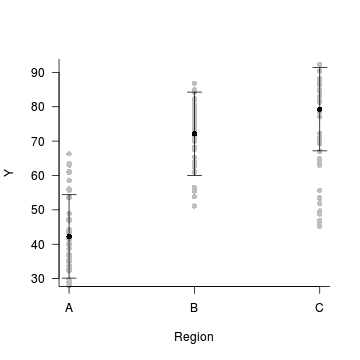
Linear mixed effects model
Step 4. plot it
with (data.nest.pred,plot.default (Region, fit,type= 'n' ,axes= F, ann= F,ylim= range (c (data.nest.pred$lower, data.nest.pred$upper))))
points (y~Region, data= data.nest, pch= 16 , col= 'grey' )
points (fit~Region, data= data.nest.pred, pch= 16 )
with (data.nest.pred, arrows (as.numeric (Region),lower,as.numeric (Region),upper, length= 0.1 , angle= 90 , code= 3 ))
axis (1 , at= 1 :3 , labels= levels (data.nest$Region))
mtext ('Region' ,1 ,line= 3 )
axis (2 ,las= 1 )
mtext ('Y' ,2 ,line= 3 )
box (bty= 'l' )
Linear mixed effects model
Linear mixed effects model
Step 4. plot it
data.nest$res <- predict (data.nest.lme, level= 0 )-
residuals (data.nest.lme)
with (data.nest.pred,plot.default (Region, fit,type= 'n' ,axes= F, ann= F,ylim= range (c (data.nest.pred$lower, data.nest.pred$upper))))
points (res~Region, data= data.nest, pch= 16 , col= 'grey' )
points (fit~Region, data= data.nest.pred, pch= 16 )
with (data.nest.pred, arrows (as.numeric (Region),lower,as.numeric (Region),upper, length= 0.1 , angle= 90 , code= 3 ))
axis (1 , at= 1 :3 , labels= levels (data.nest$Region))
mtext ('Region' ,1 ,line= 3 )
axis (2 ,las= 1 )
mtext ('Y' ,2 ,line= 3 )
box (bty= 'l' )
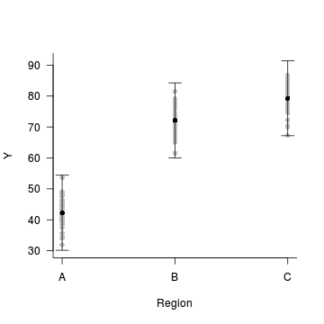
Linear mixed effects model
Linear mixed effects model
library (ggplot2)
data.nest$res <- predict (data.nest.lme, level= 0 )-
residuals (data.nest.lme)
ggplot (data.nest.pred, aes (y= fit, x= Region))+
geom_point (data= data.nest, aes (y= res), col= 'grey' ,position = position_jitter (height= 0 ))+
geom_errorbar (aes (ymin= lower, ymax= upper), width= 0.1 )+
geom_point ()+
theme_classic ()+
theme (axis.title.y= element_text (vjust= 2 ),
axis.title.x= element_text (vjust= -1 ))
Linear mixed effects model
Bayesian HMM - nested
modelString = '
model{
for (i in 1:n) {
y[i] ~ dnorm(mu[i], tau)
mu[i] <- alpha + beta.region[Region[i]] + beta.site[Sites[i]]
}
alpha ~ dnorm(0,1.0E-06)
beta.region[1] <- 0
for (i in 2:nRegion) {
beta.region[i] ~ dnorm(0, 1.0E-06)
}
for (i in 1:nSite) {
beta.site[i] ~ dnorm(0, tau.site)
}
tau <- 1/(sigma * sigma)
tau.site <- 1/(sigma.site * sigma.site)
sigma ~ dunif(0,100)
sigma.site ~ dunif(0,100)
}
'
writeLines (modelString, con= 'HMM-nest.jags' )
library (R2jags)
data.list <- with (data.nest, list (y= y, Region= as.numeric (Region),
Sites= as.numeric (Sites),
n= nrow (data.nest),
nRegion= length (unique (Region)),
nSite= length (unique (Sites))
))
data.rcb.jags <- jags (data= data.list, inits= NULL ,
param = c ('alpha' ,'beta.region' ,'beta.site' ,'sigma' ,'sigma.site' ),
model.file = 'HMM-nest.jags' ,
n.chains= 3 , n.iter= 20000 , n.burnin = 10000 ,
n.thin= 10 )Compiling model graph
Resolving undeclared variables
Allocating nodes
Graph Size: 497
Initializing modelprint (data.rcb.jags)Inference for Bugs model at "HMM-nest.jags", fit using jags,
3 chains, each with 20000 iterations (first 10000 discarded), n.thin = 10
n.sims = 3000 iterations saved
mu.vect sd.vect 2.5% 25%
alpha 42.509 7.166 28.728 37.911
beta.region[1] 0.000 0.000 0.000 0.000
beta.region[2] 29.724 10.262 9.398 23.055
beta.region[3] 36.746 10.227 16.156 30.304
beta.site[1] -8.663 7.278 -23.721 -13.053
beta.site[2] -1.112 7.267 -16.027 -5.500
beta.site[3] -11.892 7.288 -26.593 -16.333
beta.site[4] 17.270 7.249 2.359 12.816
beta.site[5] 3.069 7.304 -11.832 -1.477
beta.site[6] -11.813 7.298 -26.322 -16.532
beta.site[7] 3.021 7.268 -12.009 -1.508
beta.site[8] 9.444 7.324 -5.287 4.734
beta.site[9] 2.188 7.332 -12.683 -2.443
beta.site[10] -3.375 7.323 -18.090 -7.950
beta.site[11] 18.520 7.232 4.208 13.934
beta.site[12] 4.571 7.270 -9.885 -0.125
beta.site[13] -10.111 7.282 -24.312 -14.558
beta.site[14] -27.491 7.254 -41.878 -31.996
beta.site[15] 14.766 7.299 0.069 10.244
sigma 4.409 0.269 3.929 4.223
sigma.site 15.427 3.697 10.175 12.835
deviance 869.390 6.012 859.554 865.065
50% 75% 97.5% Rhat
alpha 42.388 46.795 57.301 1.002
beta.region[1] 0.000 0.000 0.000 1.000
beta.region[2] 29.792 36.108 50.575 1.002
beta.region[3] 36.994 42.903 57.270 1.003
beta.site[1] -8.467 -4.048 5.447 1.001
beta.site[2] -1.010 3.450 13.257 1.002
beta.site[3] -11.815 -7.213 2.385 1.002
beta.site[4] 17.440 21.858 31.416 1.002
beta.site[5] 3.236 7.799 17.353 1.002
beta.site[6] -11.752 -7.202 2.434 1.001
beta.site[7] 3.039 7.531 17.378 1.001
beta.site[8] 9.451 14.006 23.916 1.001
beta.site[9] 2.156 6.770 16.808 1.001
beta.site[10] -3.402 1.219 10.845 1.001
beta.site[11] 18.552 23.213 32.342 1.003
beta.site[12] 4.636 9.361 18.523 1.003
beta.site[13] -10.001 -5.470 4.103 1.002
beta.site[14] -27.389 -22.814 -13.516 1.002
beta.site[15] 14.887 19.382 29.256 1.002
sigma 4.396 4.576 4.963 1.001
sigma.site 14.841 17.316 24.462 1.001
deviance 868.667 872.931 883.239 1.001
n.eff
alpha 2300
beta.region[1] 1
beta.region[2] 3000
beta.region[3] 850
beta.site[1] 2100
beta.site[2] 1700
beta.site[3] 2600
beta.site[4] 2600
beta.site[5] 2200
beta.site[6] 3000
beta.site[7] 3000
beta.site[8] 3000
beta.site[9] 3000
beta.site[10] 3000
beta.site[11] 1100
beta.site[12] 1400
beta.site[13] 1500
beta.site[14] 1600
beta.site[15] 1300
sigma 3000
sigma.site 3000
deviance 3000
For each parameter, n.eff is a crude measure of effective sample size,
and Rhat is the potential scale reduction factor (at convergence, Rhat=1).
DIC info (using the rule, pD = var(deviance)/2)
pD = 18.1 and DIC = 887.5
DIC is an estimate of expected predictive error (lower deviance is better).
Bayesian HMM - nested
modelString = '
model{
for (i in 1:n) {
y[i] ~ dnorm(mu[i], tau)
mu[i] <- alpha + beta.region[Region[i]] + beta.site[Sites[i]]
}
alpha ~ dnorm(0,1.0E-06)
beta.region[1] <- 0
for (i in 2:nRegion) {
beta.region[i] ~ dnorm(0, 1.0E-06)
}
for (i in 1:nSite) {
beta.site[i] ~ dnorm(0, tau.site)
}
tau <- 1/(sigma * sigma)
tau.site <- 1/(sigma.site * sigma.site)
sigma ~ dunif(0,100)
sigma.site ~ dunif(0,100)
#Posteriors
Comp.A.B <- beta.region[1]-beta.region[2]
Comp.A.C <- beta.region[1]-beta.region[3]
Comp.B.C <- beta.region[2]-beta.region[3]
}
'
writeLines (modelString, con= 'HMM-nest.jags' )
library (R2jags)
data.list <- with (data.nest, list (y= y, Region= as.numeric (Region),
Sites= as.numeric (Sites),
n= nrow (data.nest),
nRegion= length (unique (Region)),
nSite= length (unique (Sites))
))
data.nest.jags <- jags (data= data.list, inits= NULL ,
param = c ('alpha' ,'beta.region' ,'beta.site' ,'sigma' ,'sigma.site' ,'Comp.A.B' ,'Comp.A.C' ,'Comp.B.C' ),
model.file = 'HMM-nest.jags' ,
n.chains= 3 , n.iter= 20000 , n.burnin = 10000 ,
n.thin= 10 )Compiling model graph
Resolving undeclared variables
Allocating nodes
Graph Size: 500
Initializing modelprint (data.nest.jags)Inference for Bugs model at "HMM-nest.jags", fit using jags,
3 chains, each with 20000 iterations (first 10000 discarded), n.thin = 10
n.sims = 3000 iterations saved
mu.vect sd.vect 2.5% 25%
Comp.A.B -29.689 9.893 -49.442 -35.969
Comp.A.C -37.146 9.795 -56.963 -43.390
Comp.B.C -7.457 10.180 -27.963 -13.870
alpha 42.425 6.914 28.952 38.170
beta.region[1] 0.000 0.000 0.000 0.000
beta.region[2] 29.689 9.893 9.627 23.622
beta.region[3] 37.146 9.795 18.483 30.899
beta.site[1] -8.512 6.973 -22.722 -12.792
beta.site[2] -0.974 7.029 -15.343 -5.127
beta.site[3] -11.798 6.997 -26.417 -15.934
beta.site[4] 17.377 7.043 2.942 12.896
beta.site[5] 3.160 6.986 -11.218 -1.018
beta.site[6] -11.688 7.176 -25.511 -16.278
beta.site[7] 3.139 7.154 -10.332 -1.526
beta.site[8] 9.556 7.155 -4.237 4.925
beta.site[9] 2.294 7.162 -11.576 -2.312
beta.site[10] -3.251 7.183 -17.386 -7.709
beta.site[11] 18.259 7.228 4.151 13.734
beta.site[12] 4.318 7.290 -10.145 -0.195
beta.site[13] -10.463 7.243 -24.724 -14.971
beta.site[14] -27.843 7.250 -42.152 -32.342
beta.site[15] 14.462 7.274 0.320 9.890
sigma 4.410 0.267 3.940 4.225
sigma.site 15.347 3.677 10.105 12.807
deviance 869.309 5.943 859.845 865.006
50% 75% 97.5% Rhat
Comp.A.B -29.862 -23.622 -9.627 1.001
Comp.A.C -37.119 -30.899 -18.483 1.002
Comp.B.C -7.646 -1.097 12.319 1.003
alpha 42.473 46.683 56.651 1.001
beta.region[1] 0.000 0.000 0.000 1.000
beta.region[2] 29.862 35.969 49.442 1.001
beta.region[3] 37.119 43.390 56.963 1.002
beta.site[1] -8.516 -4.234 4.860 1.001
beta.site[2] -0.938 3.408 12.639 1.001
beta.site[3] -11.850 -7.357 2.185 1.001
beta.site[4] 17.398 21.733 31.678 1.001
beta.site[5] 3.151 7.602 17.049 1.001
beta.site[6] -11.622 -7.158 2.651 1.003
beta.site[7] 3.192 7.487 17.438 1.004
beta.site[8] 9.454 13.988 23.853 1.004
beta.site[9] 2.197 6.806 16.510 1.004
beta.site[10] -3.308 1.209 10.771 1.003
beta.site[11] 18.159 22.705 32.842 1.001
beta.site[12] 4.292 8.872 19.044 1.001
beta.site[13] -10.553 -5.939 3.717 1.001
beta.site[14] -27.840 -23.341 -13.580 1.001
beta.site[15] 14.497 18.985 29.051 1.001
sigma 4.395 4.581 4.975 1.001
sigma.site 14.667 17.226 24.110 1.001
deviance 868.621 872.887 883.274 1.001
n.eff
Comp.A.B 2600
Comp.A.C 3000
Comp.B.C 800
alpha 3000
beta.region[1] 1
beta.region[2] 2600
beta.region[3] 3000
beta.site[1] 3000
beta.site[2] 3000
beta.site[3] 3000
beta.site[4] 3000
beta.site[5] 3000
beta.site[6] 680
beta.site[7] 610
beta.site[8] 520
beta.site[9] 640
beta.site[10] 710
beta.site[11] 3000
beta.site[12] 3000
beta.site[13] 3000
beta.site[14] 3000
beta.site[15] 3000
sigma 3000
sigma.site 3000
deviance 3000
For each parameter, n.eff is a crude measure of effective sample size,
and Rhat is the potential scale reduction factor (at convergence, Rhat=1).
DIC info (using the rule, pD = var(deviance)/2)
pD = 17.7 and DIC = 887.0
DIC is an estimate of expected predictive error (lower deviance is better).
Read world data examples
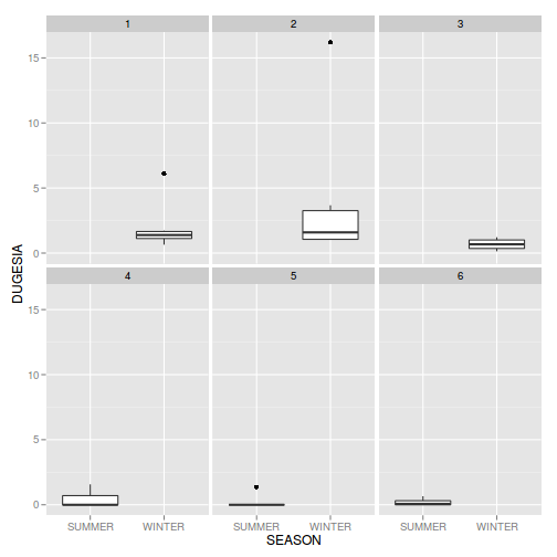
curdies <- read.csv ('../data/curdies.csv' , strip.white= T)
head (curdies)SEASON SITE DUGESIA S4DUGES 1 WINTER 1 0.6477 0.8971 2 WINTER 1 6.0962 1.5713 3 WINTER 1 1.3106 1.0700 4 WINTER 1 1.7253 1.1461 5 WINTER 1 1.4594 1.0991 6 WINTER 1 1.0576 1.0141
library (ggplot2)
ggplot (curdies, aes (y= DUGESIA, x= SEASON))+geom_boxplot ()+facet_wrap (~SITE)
plot of chunk unnamed-chunk-43
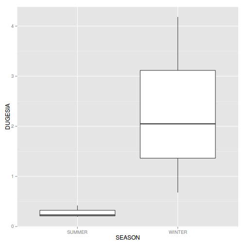
library (plyr)
curdies.ag <- ddply (curdies, ~SEASON+SITE, numcolwise (mean))
ggplot (curdies.ag, aes (y= DUGESIA, x= SEASON))+geom_boxplot ()
plot of chunk unnamed-chunk-43
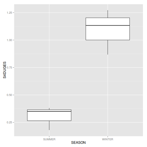
ggplot (curdies.ag, aes (y= S4DUGES, x= SEASON))+geom_boxplot ()
plot of chunk unnamed-chunk-43
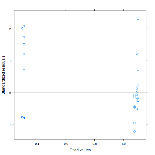
library (nlme)
curdies.lme <- lme (S4DUGES~SEASON, random= ~1 |SITE, data= curdies)
curdies.lme1 <- lme (S4DUGES~SEASON, random= ~SEASON|SITE, data= curdies)
AIC (curdies.lme, curdies.lme1) df AICcurdies.lme 4 46.43 curdies.lme1 6 50.11
anova (curdies.lme, curdies.lme1) Model df AIC BIC logLik Testcurdies.lme 1 4 46.43 52.54 -19.21
plot (curdies.lme)
plot of chunk unnamed-chunk-43
summary (curdies.lme)Linear mixed-effects model fit by REML Data: curdies AIC BIC logLik 46.43 52.54 -19.21
Random effects: Formula: ~1 | SITE (Intercept) Residual StdDev: 0.04009 0.3897
Fixed effects: S4DUGES ~ SEASON Value Std.Error DF t-value p-value (Intercept) 0.3041 0.09472 30 3.211 0.0031 SEASONWINTER 0.7868 0.13395 4 5.873 0.0042 Correlation: (Intr) SEASONWINTER -0.707
Standardized Within-Group Residuals: Min Q1 Med Q3 Max -1.2065 -0.7681 -0.2481 0.3531 2.3209
Number of Observations: 36 Number of Groups: 6
#Calculate the confidence interval for the effect size of the main effect of season
intervals (curdies.lme)Approximate 95% confidence intervals
Fixed effects: lower est. upper (Intercept) 0.1107 0.3041 0.4976 SEASONWINTER 0.4148 0.7868 1.1587 attr(,label ) [1] Fixed effects:
Random Effects: Level: SITE lower est. upper sd((Intercept)) 1.875e-07 0.04009 8571
Within-group standard error: lower est. upper 0.3026 0.3897 0.5019
#unique(confint(curdies.lme,'SEASONWINTER')[[1]])
#Examine the ANOVA table with Type I (sequential) SS
anova (curdies.lme) numDF denDF F-value p-value(Intercept) 1 30 108.5 <.0001 SEASON 1 4 34.5 0.0042
VarCorr (curdies.lme)SITE = pdLogChol(1) Variance StdDev (Intercept) 0.001607 0.04009 Residual 0.151851 0.38968
vc<-as.numeric (as.matrix (VarCorr (curdies.lme))[,1 ])
vc/sum (vc)[1] 0.01047 0.98953
curdies.lme2 <- lme (S4DUGES~1 , random= ~1 |SEASON/SITE, data= curdies)
VarCorr (curdies.lme2) Variance StdDev SEASON = pdLogChol(1)
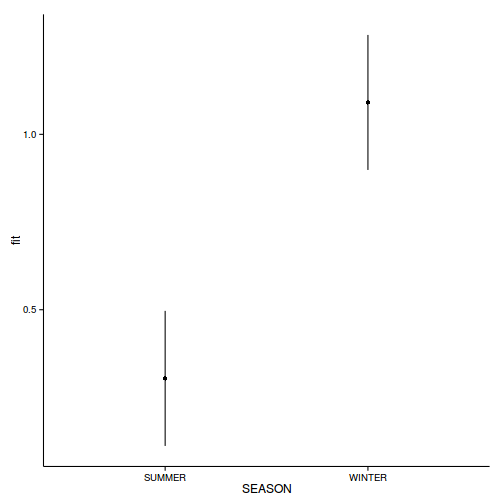
newdata <- data.frame (SEASON= levels (curdies$SEASON))
coefs <- fixef (curdies.lme)
Xmat <- model.matrix (~SEASON, data= newdata)
fit <- t (coefs %*% t (Xmat))
SE <- sqrt (diag (Xmat %*% vcov (curdies.lme) %*% t (Xmat)))
CI <- 2 *SE
#OR
CI <- qt (0.975 ,length (curdies$SEASON)-2 )*SE
newdata<- cbind (newdata, data.frame (fit= fit, se= SE,
lower= fit-CI, upper= fit+CI))
head (newdata)SEASON fit se lower upper 1 SUMMER 0.3041 0.09472 0.1116 0.4966 2 WINTER 1.0909 0.09472 0.8984 1.2834
ggplot (newdata, aes (y= fit, x= SEASON))+geom_point ()+
geom_errorbar (aes (ymin= lower, ymax= upper), width= 0 )+
theme_classic ()
plot of chunk unnamed-chunk-43
www.flutterbys.com.au/stats/downloads/data/
Format of copper.csv data file
COPPER
PLATE
DIST
WORMS
..
..
..
..
COPPER
Categorical listing of the copper treatment (control = no copper applied, week 2 = copper treatment applied in second week and week 1= copper treatment applied in first week) applied to whole plates. Factor A (between plot factor).
PLATE
Substrate provided for polychaete worm colonization on which copper treatment applied. These are the plots (Factor B). Numbers in this column represent numerical labels given to each plate.
DIST
Categorical listing for the four concentric distances from the center of the plate (source of copper treatment) with 1 being the closest and 4 the furthest. Factor C (within plot factor)
WORMS
Density (#/cm2 ) of worms measured. Response variable.
copper <- read.csv ('../data/copper.csv' , strip.white= TRUE )
Read world data examples
Factor
Effect
Effects
Treat
Fixed
2
Plate
Random
-
Dist
Fixed
3 (or 1,2,3)
Treat x Dist
Fixed
6 (or 2,..)
Plate x Treat x Dist
Random
-
Read world data examples
Questions:
Does the copper treatment effect settlement?
Does the copper treatment effect recruitment?
Does distance to copper source effect recruitment?
Assumptions
Linearity, Normality, homogeneity of variance
Independence (or a specified dependency structure)
Exploratory data analysis
copper$PLATE <- factor (copper$PLATE)
copper$DIST <- as.factor (copper$DIST)
par (mfrow= c (1 ,2 ))
boxplot (WORMS ~ COPPER*DIST, data= copper)
boxplot (sqrt (WORMS)~ COPPER*DIST, data= copper)
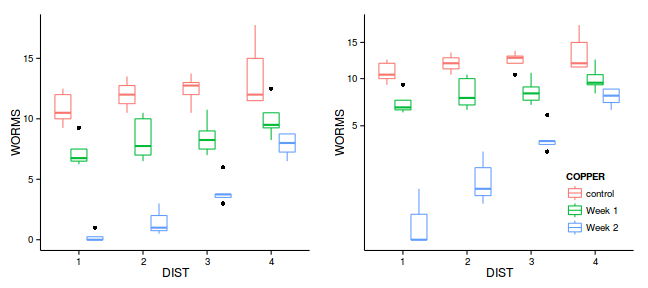
Exploratory data analysis
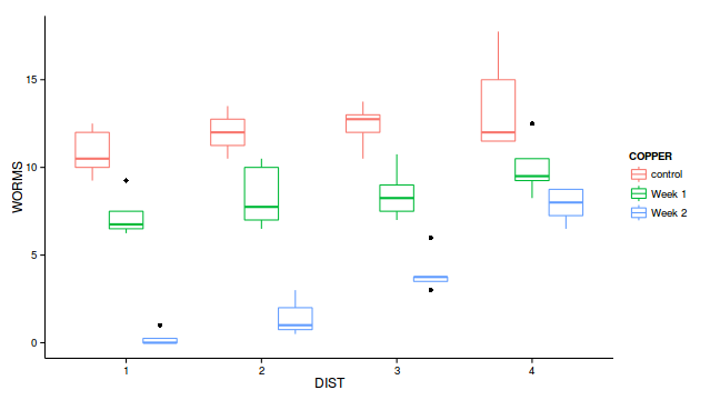
library (ggplot2)
ggplot (copper, aes (y= WORMS, x= DIST, color= COPPER)) +
geom_boxplot ()+theme_classic ()
Exploratory data analysis
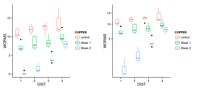
library (ggplot2)
library (gridExtra)
g1<-ggplot (copper, aes (y= WORMS, x= DIST, color= COPPER)) +
geom_boxplot ()+theme_classic ()
g2<-ggplot (copper, aes (y= WORMS, x= DIST, color= COPPER)) +
geom_boxplot ()+
scale_y_sqrt ()+theme_classic ()
grid.arrange (g1,g2, ncol= 2 )
Exploratory data analysis
library (ggplot2)
library (gridExtra)
g1<-ggplot (copper, aes (y= WORMS, x= DIST, color= COPPER)) +
geom_boxplot ()+scale_color_discrete (guide= FALSE )+
theme_classic ()
g2<-ggplot (copper, aes (y= WORMS, x= DIST, color= COPPER)) +
geom_boxplot ()+scale_y_sqrt ()+theme_classic ()+
theme (legend.position= c (1 ,0 ),
legend.justification= c (1 ,0 ))
grid.arrange (g1,g2, ncol= 2 )
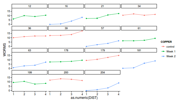
Exploratory data analysis
library (ggplot2)
ggplot (copper, aes (y= WORMS, x= as.numeric (DIST), color= COPPER)) +
facet_wrap (~PLATE)+
geom_line ()+
geom_point ()+theme_classic ()
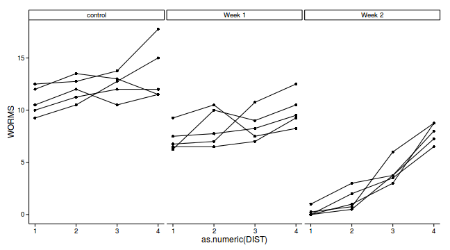
Exploratory data analysis
library (ggplot2)
ggplot (copper, aes (y= WORMS, x= as.numeric (DIST), group= PLATE)) +
facet_wrap (~COPPER)+
geom_line ()+
geom_point ()+theme_classic ()
Fit mixed effects model
library (nlme)
copper.lme <- lme (WORMS ~ COPPER*DIST, random= ~1 |PLATE,
data= copper, method= 'ML' )
plot (residuals (copper.lme, type= 'normalized' ) ~ fitted (copper.lme))
plot (residuals (copper.lme, type= 'normalized' ) ~ copper$DIST)
copper.lme1 <- update (copper.lme,
correlation= corCompSymm (form= ~1 |PLATE))
anova (copper.lme, copper.lme1) Model df AIC BIC logLik Test
copper.lme 1 14 228.3 257.6 -100.1
copper.lme1 2 15 230.3 261.7 -100.1 1 vs 2
L.Ratio p-value
copper.lme
copper.lme1 1.025e-10 1
Fit mixed effects model
library (nlme)
copper$iDIST <- as.numeric (copper$DIST)
copper.lme2 <- update (copper.lme,
correlation= corAR1 (form= ~iDIST|PLATE))
#OR
copper.lme2 <- update (copper.lme,
correlation= corAR1 (form= ~1 |PLATE))
anova (copper.lme, copper.lme2) Model df AIC BIC logLik Test
copper.lme 1 14 228.3 257.6 -100.14
copper.lme2 2 15 222.9 254.3 -96.47 1 vs 2
L.Ratio p-value
copper.lme
copper.lme2 7.352 0.0067
Fit mixed effects model
copper.lme3 <- lme (WORMS ~ COPPER*iDIST, random= ~1 |PLATE,
data= copper, method= 'ML' ,
correlation= corAR1 (form= ~1 |PLATE))
copper.lme4 <- lme (WORMS ~ COPPER*poly (iDIST,3 ),
random= ~1 |PLATE, data= copper, method= 'ML' ,
correlation= corAR1 (form= ~1 |PLATE))
anova (copper.lme2, copper.lme3, copper.lme4) Model df AIC BIC logLik Test
copper.lme2 1 15 222.9 254.3 -96.47
copper.lme3 2 9 220.5 239.3 -101.25 1 vs 2
copper.lme4 3 15 222.9 254.3 -96.47 2 vs 3
L.Ratio p-value
copper.lme2
copper.lme3 9.569 0.144
copper.lme4 9.569 0.144
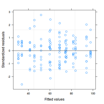
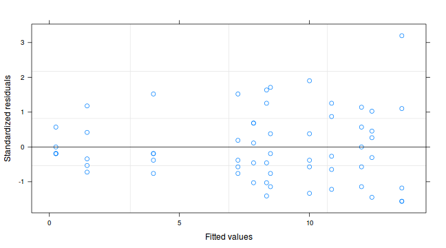
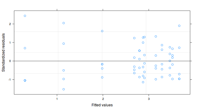
Model validation
plot (copper.lme2)
plot (residuals (copper.lme2, type= 'normalized' )~copper$DIST)
plot (residuals (copper.lme2, type= 'normalized' )~copper$COPPER)
Fit mixed effects model
copper.lme <- lme (sqrt (WORMS) ~ COPPER*DIST, random= ~1 |PLATE,
data= copper, correlation= corAR1 (form= ~1 |PLATE),
method= 'REML' )
plot (copper.lme)
plot (residuals (copper.lme, type= 'normalized' )~copper$DIST)
plot (residuals (copper.lme, type= 'normalized' )~copper$COPPER)
Summarize model
anova (copper.lme) numDF denDF F-value p-value
(Intercept) 1 36 3033.7 <.0001
COPPER 2 12 141.2 <.0001
DIST 3 36 39.7 <.0001
COPPER:DIST 6 36 15.8 <.0001summary (copper.lme)Linear mixed-effects model fit by REML
Data: copper
AIC BIC logLik
60.49 88.56 -15.24
Random effects:
Formula: ~1 | PLATE
(Intercept) Residual
StdDev: 1.415e-05 0.2873
Correlation Structure: AR(1)
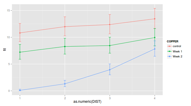
Formula: ~1 | PLATE
Parameter estimate(s):
Phi
0.3701
Fixed effects: sqrt(WORMS) ~ COPPER * DIST
Value Std.Error DF t-value
(Intercept) 3.289 0.1285 36 25.598
COPPERWeek 1 -0.603 0.1817 12 -3.320
COPPERWeek 2 -2.989 0.1817 12 -16.449
DIST2 0.172 0.1442 36 1.193
DIST3 0.229 0.1688 36 1.357
DIST4 0.378 0.1770 36 2.134
COPPERWeek 1:DIST2 0.019 0.2039 36 0.093
COPPERWeek 2:DIST2 0.672 0.2039 36 3.295
COPPERWeek 1:DIST3 -0.007 0.2387 36 -0.031
COPPERWeek 2:DIST3 1.456 0.2387 36 6.100
COPPERWeek 1:DIST4 0.091 0.2504 36 0.364
COPPERWeek 2:DIST4 2.120 0.2504 36 8.466
p-value
(Intercept) 0.0000
COPPERWeek 1 0.0061
COPPERWeek 2 0.0000
DIST2 0.2408
DIST3 0.1833
DIST4 0.0397
COPPERWeek 1:DIST2 0.9268
COPPERWeek 2:DIST2 0.0022
COPPERWeek 1:DIST3 0.9752
COPPERWeek 2:DIST3 0.0000
COPPERWeek 1:DIST4 0.7182
COPPERWeek 2:DIST4 0.0000
Correlation:
(Intr) COPPERWk1 COPPERWk2
COPPERWeek 1 -0.707
COPPERWeek 2 -0.707 0.500
DIST2 -0.561 0.397 0.397
DIST3 -0.657 0.465 0.465
DIST4 -0.689 0.487 0.487
COPPERWeek 1:DIST2 0.397 -0.561 -0.281
COPPERWeek 2:DIST2 0.397 -0.281 -0.561
COPPERWeek 1:DIST3 0.465 -0.657 -0.328
COPPERWeek 2:DIST3 0.465 -0.328 -0.657
COPPERWeek 1:DIST4 0.487 -0.689 -0.344
COPPERWeek 2:DIST4 0.487 -0.344 -0.689
DIST2 DIST3 DIST4
COPPERWeek 1
COPPERWeek 2
DIST2
DIST3 0.585
DIST4 0.463 0.653
COPPERWeek 1:DIST2 -0.707 -0.414 -0.327
COPPERWeek 2:DIST2 -0.707 -0.414 -0.327
COPPERWeek 1:DIST3 -0.414 -0.707 -0.462
COPPERWeek 2:DIST3 -0.414 -0.707 -0.462
COPPERWeek 1:DIST4 -0.327 -0.462 -0.707
COPPERWeek 2:DIST4 -0.327 -0.462 -0.707
COPPERW1:DIST2 COPPERW2:DIST2
COPPERWeek 1
COPPERWeek 2
DIST2
DIST3
DIST4
COPPERWeek 1:DIST2
COPPERWeek 2:DIST2 0.500
COPPERWeek 1:DIST3 0.585 0.293
COPPERWeek 2:DIST3 0.293 0.585
COPPERWeek 1:DIST4 0.463 0.232
COPPERWeek 2:DIST4 0.232 0.463
COPPERW1:DIST3 COPPERW2:DIST3
COPPERWeek 1
COPPERWeek 2
DIST2
DIST3
DIST4
COPPERWeek 1:DIST2
COPPERWeek 2:DIST2
COPPERWeek 1:DIST3
COPPERWeek 2:DIST3 0.500
COPPERWeek 1:DIST4 0.653 0.327
COPPERWeek 2:DIST4 0.327 0.653
COPPERW1:DIST4
COPPERWeek 1
COPPERWeek 2
DIST2
DIST3
DIST4
COPPERWeek 1:DIST2
COPPERWeek 2:DIST2
COPPERWeek 1:DIST3
COPPERWeek 2:DIST3
COPPERWeek 1:DIST4
COPPERWeek 2:DIST4 0.500
Standardized Within-Group Residuals:
Min Q1 Med Q3 Max
-1.5204 -0.7759 -0.1780 0.6235 2.4366
Number of Observations: 60
Number of Groups: 15 VarCorr (copper.lme)PLATE = pdLogChol(1)
Variance StdDev
(Intercept) 2.003e-10 1.415e-05
Residual 8.253e-02 2.873e-01
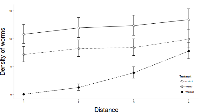
Summarize model
library (car)
interaction.plot (copper$DIST, copper$COPPER, copper$WORMS)
library (contrast)
contrast (copper.lme,
a = list (COPPER = "control" , DIST = levels (copper$DIST)),
b = list (COPPER = "Week 1" , DIST = levels (copper$DIST)))lme model parameter contrast
Contrast S.E. Lower Upper t df Pr(>|t|)
0.6032 0.1817 0.2373 0.9692 3.32 45 0.0018
0.5843 0.1817 0.2184 0.9503 3.22 45 0.0024
0.6107 0.1817 0.2447 0.9766 3.36 45 0.0016
0.5121 0.1817 0.1462 0.8781 2.82 45 0.0071contrast (copper.lme,
a = list (COPPER = "control" , DIST = levels (copper$DIST)),
b = list (COPPER = "Week 2" , DIST = levels (copper$DIST)))lme model parameter contrast
Contrast S.E. Lower Upper t df Pr(>|t|)
2.9887 0.1817 2.6228 3.355 16.45 45 0
2.3168 0.1817 1.9509 2.683 12.75 45 0
1.5327 0.1817 1.1668 1.899 8.44 45 0
0.8692 0.1817 0.5032 1.235 4.78 45 0contrast (copper.lme,
a = list (COPPER = "Week 1" , DIST = levels (copper$DIST)),
b = list (COPPER = "Week 2" , DIST = levels (copper$DIST)))lme model parameter contrast
Contrast S.E. Lower Upper t df
2.386 0.1817 2.019569 2.751 13.13 45
1.732 0.1817 1.366532 2.098 9.54 45
0.922 0.1817 0.556056 1.288 5.07 45
0.357 0.1817 -0.008912 0.723 1.97 45
Pr(>|t|)
0.0000
0.0000
0.0000
0.0556copper.lmeA <- lme (sqrt (WORMS) ~ COPPER*poly (iDIST,3 ), random= ~1 |PLATE,
data= copper, correlation= corAR1 (form= ~1 |PLATE),
method= 'REML' )
anova (copper.lmeA) numDF denDF F-value p-value
(Intercept) 1 36 3033.7 <.0001
COPPER 2 12 141.2 <.0001
poly(iDIST, 3) 3 36 39.7 <.0001
COPPER:poly(iDIST, 3) 6 36 15.8 <.0001round (summary (copper.lmeA)$tTable,3 ) Value Std.Error DF
(Intercept) 3.483 0.084 36
COPPERWeek 1 -0.578 0.119 12
COPPERWeek 2 -1.927 0.119 12
poly(iDIST, 3)1 1.031 0.512 36
poly(iDIST, 3)2 -0.045 0.417 36
poly(iDIST, 3)3 0.179 0.360 36
COPPERWeek 1:poly(iDIST, 3)1 0.214 0.724 36
COPPERWeek 2:poly(iDIST, 3)1 6.186 0.724 36
COPPERWeek 1:poly(iDIST, 3)2 0.154 0.590 36
COPPERWeek 2:poly(iDIST, 3)2 -0.016 0.590 36
COPPERWeek 1:poly(iDIST, 3)3 0.147 0.508 36
COPPERWeek 2:poly(iDIST, 3)3 -0.202 0.508 36
t-value p-value
(Intercept) 41.379 0.000
COPPERWeek 1 -4.852 0.000
COPPERWeek 2 -16.185 0.000
poly(iDIST, 3)1 2.015 0.051
poly(iDIST, 3)2 -0.108 0.915
poly(iDIST, 3)3 0.498 0.622
COPPERWeek 1:poly(iDIST, 3)1 0.295 0.769
COPPERWeek 2:poly(iDIST, 3)1 8.549 0.000
COPPERWeek 1:poly(iDIST, 3)2 0.261 0.795
COPPERWeek 2:poly(iDIST, 3)2 -0.028 0.978
COPPERWeek 1:poly(iDIST, 3)3 0.290 0.774
COPPERWeek 2:poly(iDIST, 3)3 -0.397 0.694library (multcomp)
summary (glht (copper.lme, linfct= mcp (COPPER= 'Tukey' )))
     Simultaneous Tests for General Linear Hypotheses

Multiple Comparisons of Means: Tukey Contrasts


Fit: lme.formula(fixed = sqrt(WORMS) ~ COPPER * DIST, data = copper,
    random = ~1 | PLATE, correlation = corAR1(form = ~1 | PLATE),
    method = "REML")

Linear Hypotheses:
                      Estimate Std. Error z value
Week 1 - control == 0   -0.603      0.182   -3.32
Week 2 - control == 0   -2.989      0.182  -16.45
Week 2 - Week 1 == 0    -2.386      0.182  -13.13
                      Pr(>|z|)
Week 1 - control == 0   0.0025 **
Week 2 - control == 0   <1e-04 ***
Week 2 - Week 1 == 0    <1e-04 ***
---
Signif. codes:
0 '***' 0.001 '**' 0.01 '*' 0.05 '.' 0.1 ' ' 1
(Adjusted p values reported -- single-step method)
summary (glht (copper.lme, linfct= mcp (DIST= 'Tukey' )))
     Simultaneous Tests for General Linear Hypotheses

Multiple Comparisons of Means: Tukey Contrasts


Fit: lme.formula(fixed = sqrt(WORMS) ~ COPPER * DIST, data = copper,
    random = ~1 | PLATE, correlation = corAR1(form = ~1 | PLATE),
    method = "REML")

Linear Hypotheses:
           Estimate Std. Error z value Pr(>|z|)
2 - 1 == 0   0.1720     0.1442    1.19     0.63
3 - 1 == 0   0.2290     0.1688    1.36     0.52
4 - 1 == 0   0.3778     0.1770    2.13     0.14
3 - 2 == 0   0.0571     0.1442    0.40     0.98
4 - 2 == 0   0.2058     0.1688    1.22     0.61
4 - 3 == 0   0.1487     0.1442    1.03     0.73
(Adjusted p values reported -- single-step method)
Bayesian
modelString="
model {
#Likelihood
for (i in 1:n) {
y[i]~dnorm(mu[i],tau)
mu[i] <- alpha0 + alpha[A[i]]+beta[Block[i]] + C.gamma[C[i]] + AC.gamma[A[i],C[i]]
}
#Priors
alpha0 ~ dnorm(0, 1.0E-6)
alpha[1] <- 0
for (i in 2:nA) {
alpha[i] ~ dnorm(0, 1.0E-6) #prior
AC.gamma[i,1] <- 0
}
for (i in 1:nBlock) {
beta[i] ~ dnorm(0, tau.B) #prior
}
C.gamma[1] <- 0
for (i in 2:nC) {
C.gamma[i] ~ dnorm(0, 1.0E-6)
AC.gamma[1,i] <- 0
}
AC.gamma[1,1] <- 0
for (i in 2:nA) {
for (j in 2:nC) {
AC.gamma[i,j] ~ dnorm(0, 1.0E-6)
}
}
sigma ~ dunif(0, 100)
tau <- 1 / (sigma * sigma)
sigma.B ~ dunif(0, 100)
tau.B <- 1 / (sigma.B * sigma.B)
}
"
writeLines (modelString,con= "../BUGSscripts/splitPlot.jags" )
data.list <- with (copper,
list (y= sqrt (WORMS),
Block= as.numeric (PLATE),
A= as.numeric (COPPER),
C= as.numeric (DIST),
n= nrow (copper),
nA = length (levels (COPPER)),
nC = length (levels (DIST)),
nBlock = length (levels (PLATE))
)
)
params <- c ("alpha0" ,"alpha" ,'C.gamma' ,'AC.gamma' ,"sigma" ,"sigma.B" )
burnInSteps = 3000
nChains = 3
numSavedSteps = 3000
thinSteps = 10
nIter = burnInSteps+ceiling ((numSavedSteps * thinSteps)/nChains)
library (R2jags)
rnorm (1 )[1] -1.53
jags.f.time <- system.time (
data.r2jags.f <- jags (data= data.list,
inits= NULL ,
parameters.to.save= params,
model.file= "../BUGSscripts/splitPlot.jags" ,
n.chains= nChains,
n.iter= nIter,
n.burnin= burnInSteps,
n.thin= thinSteps
)
) Compiling model graph Resolving undeclared variables Allocating nodes Graph Size: 349
Initializing model
print (data.r2jags.f)Inference for Bugs model at ../BUGSscripts/splitPlot.jags , fit using jags, 3 chains, each with 13000 iterations (first 3000 discarded), n.thin = 10 n.sims = 3000 iterations saved mu.vect sd.vect 2.5% 25% AC.gamma[1,1] 0.000 0.000 0.000 0.000 AC.gamma[2,1] 0.000 0.000 0.000 0.000 AC.gamma[3,1] 0.000 0.000 0.000 0.000 AC.gamma[1,2] 0.000 0.000 0.000 0.000 AC.gamma[2,2] 0.014 0.256 -0.487 -0.157 AC.gamma[3,2] 0.670 0.250 0.177 0.502 AC.gamma[1,3] 0.000 0.000 0.000 0.000 AC.gamma[2,3] -0.009 0.247 -0.499 -0.169 AC.gamma[3,3] 1.457 0.255 0.960 1.282 AC.gamma[1,4] 0.000 0.000 0.000 0.000 AC.gamma[2,4] 0.091 0.249 -0.410 -0.071 AC.gamma[3,4] 2.119 0.252 1.620 1.955 C.gamma[1] 0.000 0.000 0.000 0.000 C.gamma[2] 0.172 0.180 -0.177 0.050 C.gamma[3] 0.229 0.178 -0.126 0.111 C.gamma[4] 0.378 0.174 0.028 0.260 alpha[1] 0.000 0.000 0.000 0.000 alpha[2] -0.600 0.197 -0.993 -0.727 alpha[3] -2.988 0.199 -3.392 -3.119 alpha0 3.289 0.140 3.014 3.198 sigma 0.278 0.032 0.224 0.255 sigma.B 0.111 0.065 0.010 0.064 deviance 14.470 8.355 -0.458 8.584 50% 75% 97.5% Rhat n.eff AC.gamma[1,1] 0.000 0.000 0.000 1.000 1 AC.gamma[2,1] 0.000 0.000 0.000 1.000 1 AC.gamma[3,1] 0.000 0.000 0.000 1.000 1 AC.gamma[1,2] 0.000 0.000 0.000 1.000 1 AC.gamma[2,2] 0.012 0.188 0.523 1.001 3000 AC.gamma[3,2] 0.665 0.838 1.156 1.001 3000 AC.gamma[1,3] 0.000 0.000 0.000 1.000 1 AC.gamma[2,3] -0.008 0.159 0.469 1.002 1100 AC.gamma[3,3] 1.453 1.624 1.971 1.002 1500 AC.gamma[1,4] 0.000 0.000 0.000 1.000 1 AC.gamma[2,4] 0.095 0.254 0.577 1.001 2400 AC.gamma[3,4] 2.117 2.284 2.619 1.001 3000 C.gamma[1] 0.000 0.000 0.000 1.000 1 C.gamma[2] 0.172 0.292 0.529 1.001 3000 C.gamma[3] 0.230 0.350 0.568 1.002 2000 C.gamma[4] 0.382 0.491 0.717 1.001 3000 alpha[1] 0.000 0.000 0.000 1.000 1 alpha[2] -0.603 -0.470 -0.223 1.001 3000 alpha[3] -2.986 -2.852 -2.610 1.001 2800 alpha0 3.288 3.382 3.562 1.001 3000 sigma 0.276 0.297 0.349 1.001 3000 sigma.B 0.106 0.150 0.252 1.029 180 deviance 14.233 19.709 32.181 1.003 970
For each parameter, n.eff is a crude measure of effective sample size, and Rhat is the potential scale reduction factor (at convergence, Rhat=1).
DIC info (using the rule, pD = var(deviance)/2) pD = 34.9 and DIC = 49.3 DIC is an estimate of expected predictive error (lower deviance is better).