Linear models
\[ \begin{align*} y_{i} &= \beta_0 + \beta_1 \times x_{i} + \varepsilon_i\\ \epsilon_i&\sim\mathcal{N}(0, \sigma^2) \\ \end{align*} \]

\[ \begin{align*} y_{i} &= \beta_0 + \beta_1 \times x_{i} + \varepsilon_i\\ \epsilon_i&\sim\mathcal{N}(0, \sigma^2) \\ \end{align*} \]

\(y \sim{} N(\mu, \sigma^2)\\ \mu = \beta_0 + \beta_1 x_1 + \beta_2 x_2\)
Polynomial
\(y \sim{} N(\mu, \sigma^2)\\ \mu = \beta_0 + \beta_1 x + \beta_2 x^2 + \beta_2 x^3\)
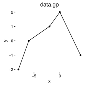
> data.gp.lm <- lm(y~x+I(x^2), data=data.gp)
> #OR
> data.gp.lm <- lm(y~poly(x,2), data=data.gp)
> summary(data.gp.lm)
Call:
lm(formula = y ~ poly(x, 2), data = data.gp)

Residuals:
        1         2         3         4         5
-0.008658  0.129870 -0.580087  0.571429 -0.112554

Coefficients:
              Estimate Std. Error t value Pr(>|t|)
(Intercept) -3.885e-16  2.632e-01   0.000   1.0000
poly(x, 2)1  1.047e+00  5.885e-01   1.779   0.2171
poly(x, 2)2 -2.865e+00  5.885e-01  -4.869   0.0397 *
---
Signif. codes:  0 '***' 0.001 '**' 0.01 '*' 0.05 '.' 0.1 ' ' 1

Residual standard error: 0.5885 on 2 degrees of freedom
Multiple R-squared:  0.9307,    Adjusted R-squared:  0.8615
F-statistic: 13.44 on 2 and 2 DF, p-value: 0.06926> newdata <- data.frame(x=seq(min(data.gp$x),
+ max(data.gp$x), l=100))
> pred <- predict(data.gp.lm, newdata=newdata,
+ interval='confidence')
> newdata <- cbind(newdata,pred)
> head(newdata) x fit lwr upr
1 -8.000000 -1.991342 -4.220269 0.2375849
2 -7.878788 -1.859425 -4.011062 0.2922128
3 -7.757576 -1.729972 -3.808290 0.3483463
4 -7.636364 -1.602984 -3.612054 0.4060865
5 -7.515152 -1.478460 -3.422451 0.4655306
6 -7.393939 -1.356401 -3.239573 0.5267699> ggplot(newdata, aes(y=fit, x=x))+
+ geom_point(data=data.gp, aes(y=y))+
+ geom_ribbon(aes(ymin=lwr,ymax=upr),fill='blue',alpha=0.5)+
+ geom_line()+
+ theme_classic()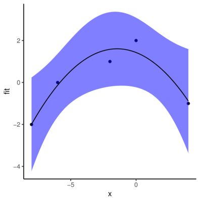
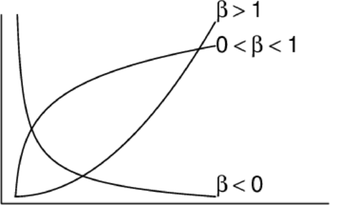
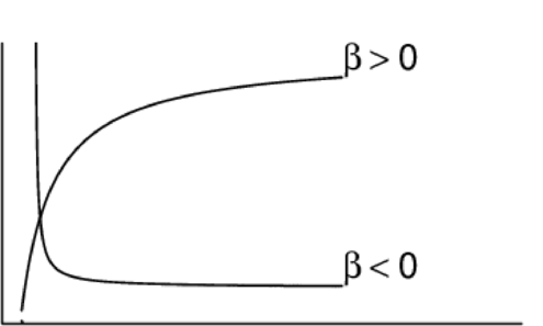
Power (\(y = \alpha x^\beta\))
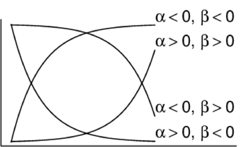
Exponential Curve (\(y = \alpha e^{\beta x}\))

Asymptotic exponential \(y = \alpha + (\beta - \alpha) e^{-e^{\gamma} x}\) 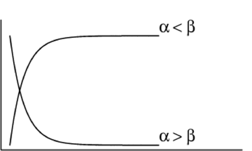
Michaelis-Menton (\(y = \frac{\alpha x}{\beta + x}\))
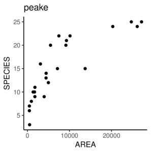
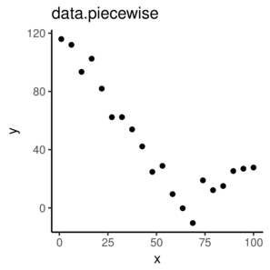
> nls(y ~ a * exp(b*x), start=list(a=1, b=1), data=data)> nls(y ~ SSasymp(AREA,a,b,c), start=list(a=1, b=1), data=data)> data.piecewise <- read.csv('../data/data.piecewise.csv')
> ggplot(data.piecewise, aes(y=y, x=x))+geom_point()+
+ theme_classic()

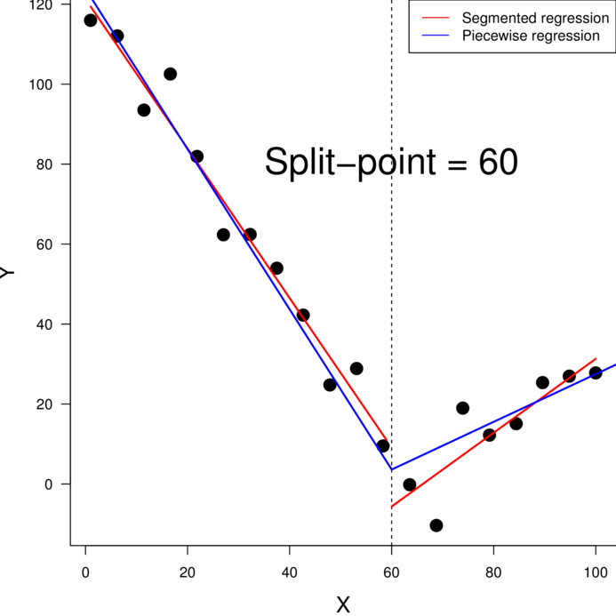
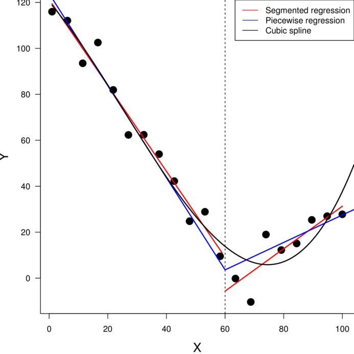
> library(splines)\(y \sim{} N(\mu, \sigma^2)\\ \mu = \beta_0 + \beta_1 x_1 + \beta_2 x_2\)
\(y \sim{} Pois(\mu, \sigma^2)\\ g(\mu) = \beta_0 + \beta_1 x_1 + \beta_2 x_2\)
\(y \sim{} Pois(\mu, \sigma^2)\\ g(\mu) = \beta_0 + \beta_1 x_1 + \beta_2 x_2\)
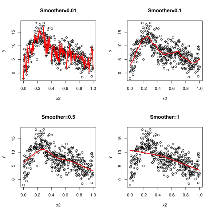
\(y \sim{} Pois(\mu, \sigma^2)\\ g(\mu) = \beta_0 + f(x_1) + f(x_2)\)
> library(mgcv)
> dat.gam <- gam(y~s(x1)+s(x2)+s(x3), data=dat)
> summary(dat.gam)
Family: gaussian
Link function: identity

Formula:
y ~ s(x1) + s(x2) + s(x3)

Parametric coefficients:
            Estimate Std. Error t value Pr(>|t|)
(Intercept)   7.7281     0.1027   75.27   <2e-16 ***
---
Signif. codes:  0 '***' 0.001 '**' 0.01 '*' 0.05 '.' 0.1 ' ' 1

Approximate significance of smooth terms:
        edf Ref.df      F p-value
s(x1) 2.821  3.509 78.087  <2e-16 ***
s(x2) 8.208  8.829 84.163  <2e-16 ***
s(x3) 1.000  1.000  0.009   0.923
---
Signif. codes:  0 '***' 0.001 '**' 0.01 '*' 0.05 '.' 0.1 ' ' 1

R-sq.(adj) =  0.725   Deviance explained = 73.3%
GCV = 4.3588 Scale est. = 4.2168 n = 400> plot(dat.gam, pages=1)
> plot(dat.gam, select=2, shade=TRUE)
> library(mgcv)
> dat.gam <- gam(y~s(x2,x3), data=dat)
> summary(dat.gam)
Family: gaussian
Link function: identity

Formula:
y ~ s(x2, x3)

Parametric coefficients:
            Estimate Std. Error t value Pr(>|t|)
(Intercept)   7.7281     0.1346   57.43   <2e-16 ***
---
Signif. codes:  0 '***' 0.001 '**' 0.01 '*' 0.05 '.' 0.1 ' ' 1

Approximate significance of smooth terms:
           edf Ref.df     F p-value
s(x2,x3) 25.92  28.43 15.94  <2e-16 ***
---
Signif. codes:  0 '***' 0.001 '**' 0.01 '*' 0.05 '.' 0.1 ' ' 1

R-sq.(adj) =  0.528   Deviance explained = 55.8%
GCV = 7.7651 Scale est. = 7.2425 n = 400> plot(dat.gam, pages=1, scheme=2)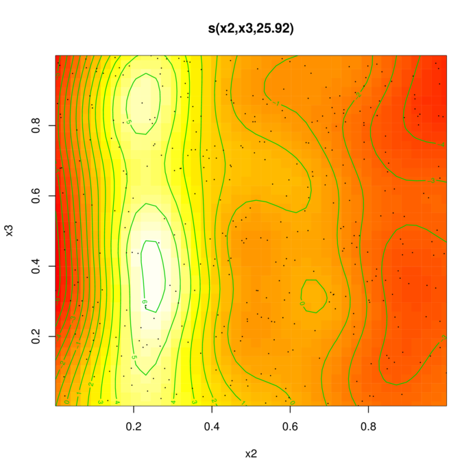
> vis.gam(dat.gam, theta=35)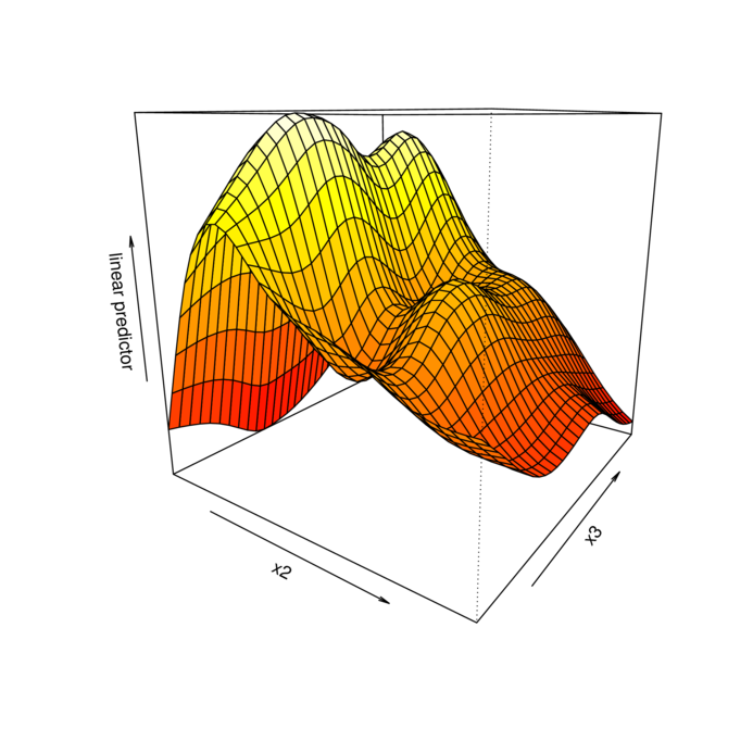
> vis.gam(dat.gam, theta=35, se=2)
> ## wq <- read.csv('../data/wq.csv', strip.white=TRUE)
> ## library(tidyr)
> ## wq <- wq %>% select(LATITUDE,LONGITUDE,reef.alias,Water_Samples,Region,Subregion,Season,waterYear,Date,Mnth,Dt.num,Source,Measure,Value) %>%
> ##     #filter(Water_Samples=='AIMS', Source=='AIMS Niskin') %>%
> ##         filter(Source=='AIMS Niskin') %>%
> ##         spread(key=Measure,value=Value)
> ## nms <- colnames(wq)
> ## nms=gsub('\\.wm','',nms)
> ## colnames(wq) <- nms
> ## write.csv(wq,file='../data/aims.wq.csv', row.names=FALSE, quote=FALSE)
> wq=read.csv(file='../data/aims.wq.csv', strip.white=TRUE)
> head(wq)
LATITUDE LONGITUDE reef.alias Water_Samples Region Subregion Season waterYear 1 -16.11152 145.4833 Cape Tribulation AIMS Wet Tropics Barron Daintree Dry 2008 2 -16.11383 145.4827 Cape Tribulation AIMS Wet Tropics Barron Daintree Wet 2008 3 -16.11261 145.4844 Cape Tribulation AIMS Wet Tropics Barron Daintree Dry 2009 4 -16.11308 145.4868 Cape Tribulation AIMS Wet Tropics Barron Daintree Wet 2009 5 -16.11343 145.4835 Cape Tribulation AIMS Wet Tropics Barron Daintree Dry 2009 6 -16.11306 145.4846 Cape Tribulation AIMS Wet Tropics Barron Daintree Dry 2010 Date Mnth Dt.num Source CDOM_443 CHL_TSS DIN DIP DOC_DON DOC_DOP 1 2007-10-14 10 2007.784 AIMS Niskin NA 0.3101798 NA 3.2430236 9.894332 249.5793 2 2008-03-30 3 2008.243 AIMS Niskin NA 0.1077403 1.7603107 0.0000000 18.838502 164.1689 3 2008-10-12 10 2008.779 AIMS Niskin NA 0.1927524 1.8912551 8.4301889 10.247938 232.2605 4 2009-02-26 2 2009.153 AIMS Niskin NA 0.4841206 1.5700109 0.2818657 8.853276 138.2857 5 2009-06-15 6 2009.452 AIMS Niskin NA 0.2699770 0.9340067 3.3818466 35.173595 143.7499 6 2009-10-12 10 2009.778 AIMS Niskin NA 0.2303556 0.8530959 2.8842803 10.913727 334.8760 DOC DON_DOP DON DOP DRIFTCHL_UGPERL DRIFTPHAE_UGPERL Dt.num.1 Dtt.num 1 568.7456 25.371405 58.39177 2.360146 0.2348550 0.1066725 2007.784 1192330200 2 800.0811 8.672342 42.59066 5.676724 0.3407700 0.2378625 2008.243 1206843900 3 665.5129 21.385520 66.56530 -3.369768 0.3229300 0.1444425 2008.779 1223763420 4 790.8947 15.773521 89.86323 6.108445 0.3026219 0.1158813 2009.153 1235609580 5 709.3114 4.218696 21.04308 5.245931 0.3904875 0.1867100 2009.452 1245043620 6 703.8190 31.476436 65.64792 2.429785 0.3303821 0.1286239 2009.778 1255308780 HAND_NH4 NH4 NO2 NO3 NOx_PO4 NOx PN_CHL PN_PP PN_SHIM PN_TSS 1 NA 3.321632 0.0000000 0.8225237 0.2336054 0.8300237 50.81076 5.457474 18.99411 0.017091541 2 1.657928 1.013287 0.0000000 0.0000000 Inf 0.0100000 70.97502 4.841050 29.22387 0.007517002 3 1.187635 2.984873 0.0000000 0.2744196 0.1661957 0.2819196 43.20272 5.852297 13.21873 0.008352101 4 0.244650 5.136503 0.0000000 1.2644041 Inf 1.2675291 32.14920 5.035881 14.93224 0.014976245 5 0.186260 3.343649 0.1400100 0.6533917 0.2072996 0.7934017 40.25010 5.801272 18.73589 0.011240255 6 0.401402 2.223354 0.1245889 0.2553082 0.1354893 0.3798971 31.42818 4.031699 14.72265 0.007149731 PN PO4 POC_CHL POC_PN POC_PP POC_TSS POC PP_CHL PP_TSS 1 9.556838 3.2430236 643.2646 13.802976 78.17430 0.28442285 126.47385 9.073836 0.002787327 2 17.876092 0.0000000 594.1710 8.211349 39.91906 0.06276370 147.34368 13.775650 0.001460411 3 13.877616 8.4301889 320.9770 7.611680 43.86293 0.06193767 103.58926 7.352966 0.001423642 4 9.648177 0.2818657 300.8186 9.477119 46.88621 0.14314580 89.97550 6.429233 0.003094262 5 13.335427 3.3818466 334.7438 8.455543 48.09479 0.09331987 110.71416 6.769279 0.001870709 6 10.168986 2.8842803 274.4056 8.900616 34.94283 0.06257516 88.06501 7.830029 0.001787518 PP Salinity SECCHI_DEPTH SI_NOx SI_PO4 SI TDN TDP TN_TP 1 2.025051 NA 11.0 5345.75834 20.99143 70.47872 62.53592 5.603170 9.567956 2 3.678694 NA 4.0 32763.52291 Inf 327.63523 43.60394 5.676724 6.958258 3 2.371837 NA 3.8 8925.66237 42.09525 119.92590 69.82460 5.060421 11.240651 4 1.922521 NA 6.0 5725.21940 Inf 196.88465 96.26414 6.390311 13.392960 5 2.336996 NA 6.0 391.95711 59.47313 160.96946 25.18013 8.627777 3.586795 6 2.557138 NA 11.0 81.68518 10.50605 29.76851 68.01086 5.314065 10.043426 TotalN TotalP TSS_MGPERL 1 72.09276 7.628221 1.052500 2 61.48004 9.355418 3.120000 3 83.70221 7.432258 1.695000 4 105.91231 8.312832 0.761250 5 38.51556 10.964774 1.505000 6 78.17984 7.871202 1.432857
> wq = wq %>% mutate(Date=as.Date(Date))Error in eval(expr, envir, enclos): could not find function "%>%"> ggplot(wq, aes(y=NOx, x=Date)) + geom_point()> ggplot(wq, aes(y=NOx, x=Date)) + geom_point() +
+ scale_y_log10()> ggplot(wq, aes(y=NOx, x=Date)) + geom_point() +
+ geom_smooth() +
+ scale_y_log10()> ggplot(wq, aes(y=NOx, x=Date)) +
+ geom_point() +
+ geom_smooth() +
+ scale_y_log10() +
+ facet_wrap(~Subregion)> library(lubridate)
> library(mgcv)
> wq = wq %>% mutate(Dt.num = decimal_date(Date))Error in eval(expr, envir, enclos): could not find function "%>%"> wq.gamm <- gamm(NOx ~ s(Dt.num), random=list(reef.alias=~1), data=wq)
>
> gam.check(wq.gamm$gam, pch=19)> library(MASS)
> wq.gamm <- gamm(NOx ~ s(Dt.num), random=list(reef.alias=~1), data=wq, family=gaussian)
> wq.gamm <- gamm(NOx ~ s(Dt.num), random=list(reef.alias=~1), data=wq,
+ family=negative.binomial(3))Maximum number of PQL iterations: 20
> wq.gamm <- gamm(NOx ~ s(Dt.num), random=list(reef.alias=~1), data=wq, family=quasipoisson)Maximum number of PQL iterations: 20
> wq.gamm <- gamm(NOx ~ s(Dt.num), random=list(reef.alias=~1), data=wq, family=neg.bin(theta=3))Maximum number of PQL iterations: 20
> AIC(wq.gamm)Error in UseMethod("logLik"): no applicable method for 'logLik' applied to an object of class "c('gamm', 'list')"> gam.check(wq.gamm$gam, pch=19)> plot(wq.gamm$gam)> wq.gamm <- gamm(NOx ~ s(Dt.num)+
+ s(Mnth,bs='cc',k=5,fx=F),
+ knots=list(Mnth=seq(1,12,length=5)),
+ random=list(reef.alias=~1),
+ family=neg.bin(theta=3),
+ data=wq)Maximum number of PQL iterations: 20
> gam.check(wq.gamm$gam, pch=19)> plot(wq.gamm$gam, page=1, seWithMean=TRUE,scale=0)> wq.gamm <- gamm(NOx ~ s(Dt.num,by=Subregion)+
+ s(Mnth,bs='cc',k=5,fx=F,by=Subregion),
+ knots=list(Mnth=seq(1,12,length=5)),
+ random=list(reef.alias=~1),
+ family=neg.bin(theta=3),
+ data=wq)Maximum number of PQL iterations: 20
> wq.gamm <- gamm(NOx ~ s(Dt.num,by=Subregion)+
+                     s(Mnth,bs='cc',k=5,fx=F,by=Subregion),
+                 knots=list(Mnth=seq(1,12,length=5)),
+                 random=list(reef.alias=~1),
+                 family=Tweedie(2),
+                 data=wq)
Maximum number of PQL iterations: 20
> #control=list(maxIter=100)
> gam.check(wq.gamm$gam, pch=19)> plot(wq.gamm$gam, page=1, seWithMean=TRUE,scale=0)> summary(wq.gamm$gam)Family: Tweedie(2) Link function: log
Formula: NOx ~ s(Dt.num, by = Subregion) + s(Mnth, bs = “cc”, k = 5, fx = F, by = Subregion)
Parametric coefficients: Estimate Std. Error t value Pr(>|t|) (Intercept) 0.1570 0.1348 1.165 0.245
Approximate significance of smooth terms: edf Ref.df F p-value
s(Dt.num):SubregionBarron Daintree 5.257e+00 5.257 22.653 < 2e-16 s(Dt.num):SubregionBurdekin 5.835e+00 5.835 16.771 < 2e-16 s(Dt.num):SubregionJohnstone Russell Mulgrave 2.890e+00 2.890 11.252 6.90e-07 s(Dt.num):SubregionMackay Whitsunday 2.587e+00 2.587 4.418 0.00737 s(Dt.num):SubregionTully Herbert 3.728e+00 3.728 12.837 2.91e-09 s(Mnth):SubregionBarron Daintree 3.779e-06 3.000 0.000 0.51470
s(Mnth):SubregionBurdekin 1.171e+00 3.000 0.815 0.11885
s(Mnth):SubregionJohnstone Russell Mulgrave 7.294e-05 3.000 0.000 0.35755
s(Mnth):SubregionMackay Whitsunday 2.226e+00 3.000 10.055 1.37e-07 s(Mnth):SubregionTully Herbert 1.875e+00 3.000 2.368 0.01518
— Signif. codes: 0 ‘’ 0.001 ’’ 0.01 ’’ 0.05 ‘.’ 0.1 ‘’ 1
R-sq.(adj) = -0.00133
Scale est. = 1.1397 n = 568
> newdata = expand.grid(Dt.num = seq(min(wq$Dt.num), max(wq$Dt.num), len=100),
+     Mnth=c(2,6),
+     Subregion=levels(wq$Subregion))
> Q=qt(0.975, df=wq.gamm$gam$df.resid)
> pred = predict(wq.gamm$gam, newdata=newdata, se.fit=TRUE, type='response')
> newdata = cbind(newdata, fit=pred$fit, lower=pred$fit-pred$se.fit,
+     upper=pred$fit+pred$se.fit)
>
>
>
> ggplot(newdata, aes(y=fit, x=date_decimal(Dt.num), color=factor(Mnth))) +
+     geom_line() +
+         geom_ribbon(aes(ymin=lower, ymax=upper, fill=factor(Mnth)),
+                     color=NA,alpha=0.3)+
+             facet_wrap(~Subregion, scales='free')+
+                 theme_classic() +
+                     theme(axis.line.x=element_line(),
+ axis.line.y=element_line())> ggplot(newdata, aes(y=fit, x=date_decimal(Dt.num), color=factor(Mnth))) +
+ geom_line() +
+ geom_ribbon(aes(ymin=lower, ymax=upper, fill=factor(Mnth)),
+ color=NA,alpha=0.3)+
+ facet_wrap(~Subregion, scales='free')+
+ theme_classic() +
+ theme(axis.line.x=element_line(),
+ axis.line.y=element_line(),
+ axis.title.x=element_blank(),
+ strip.background=element_blank())
single models fail to capture complexity
Feature complexity
(Multi)collinearity
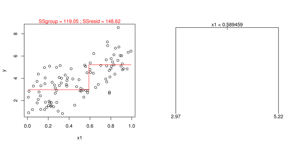
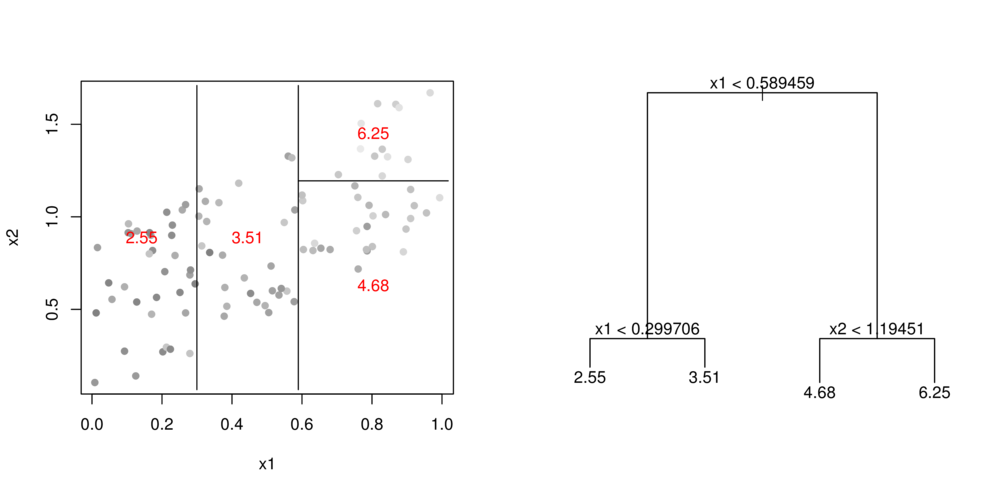
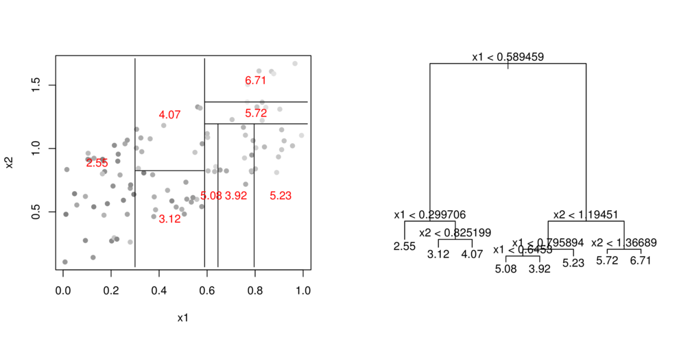
CART

- split (**partition**) data up into __major__ chunks


> library(tree)> library(rpart)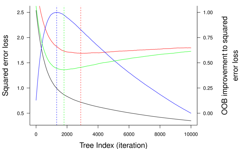


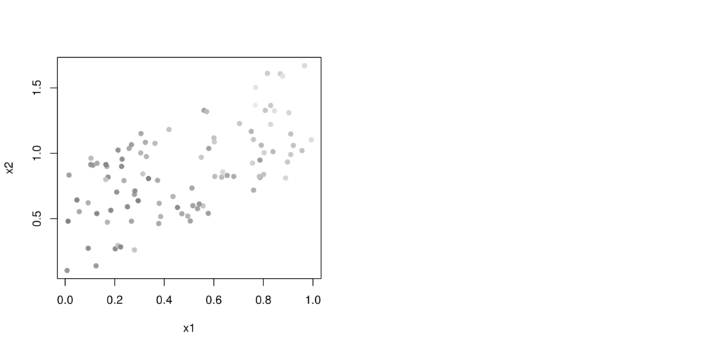
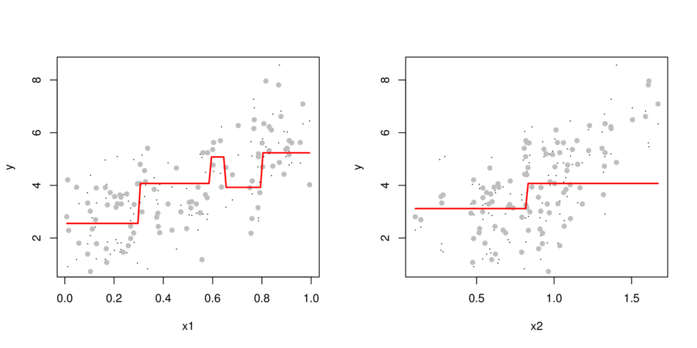
   var  rel.inf
x1  x1 55.05679
x2 x2 44.94321[1] 0.5952246