Non-linear models
Power (\(y = \alpha x^\beta\))

Exponential (\(y = \alpha e^{\beta x}\))
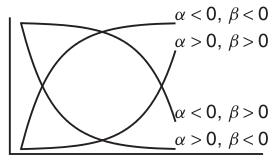
Power (\(y = \alpha x^\beta\))
Exponential (\(y = \alpha e^{\beta x}\))
Asymptotic exponential
\(y = \alpha + (\beta - \alpha) e^{-e^{\gamma} x}\) 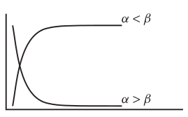
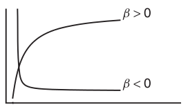
Michaelis-Menton (\(y = \frac{\alpha x}{\beta + x}\))
peake <- read.table("../data/peake.csv", header = T,
    sep = ",", strip.white = T)
head(peake)
AREA SPECIES INDIV1 516.0 3 18 2 469.1 7 60 3 462.2 6 57 4 938.6 8 100 5 1357.2 10 48 6 1773.7 9 118
## @knitr Q4-a, fig.height=5.0, fig.width=5.0
library(car)
scatterplot(SPECIES ~ AREA, data = peake)
## @knitr Q4-2a
peake.lm <- lm(SPECIES ~ AREA + I(AREA^2), data = peake)


## @knitr Q4-2b
peake.nls <- nls(SPECIES ~ alpha * AREA^beta, data = peake,
    start = list(alpha = 0.1, beta = 1))


## @knitr Q4-2c
peake.nls1 <- nls(SPECIES ~ SSasymp(AREA, a, b, c),
    data = peake)


## @knitr Q4-3a
peake.lmLin <- lm(SPECIES ~ AREA, data = peake)
# calculate AIC for the linear model
AIC(peake.lmLin)
[1] 141.1
# calculate mean-square residual of the linear
# model
deviance(peake.lmLin)/df.residual(peake.lmLin)
[1] 14.13
AIC(peake.lm)[1] 129.5
# calculate mean-square residual of the power model
deviance(peake.lm)/df.residual(peake.lm)
[1] 8.602
# assess the goodness of fit between linear and
# polynomial models
anova(peake.lmLin, peake.lm)
Analysis of Variance Table
Model 1: SPECIES ~ AREA Model 2: SPECIES ~ AREA + I(AREA^2) Res.Df RSS Df Sum of Sq F Pr(>F)
1 23 325
2 22 189 1 136 15.8 0.00064 * — Signif. codes:
0 ’ 0.001 ’’ 0.01 ’
0.05 ’.’ 0.1 ’ ’ 1
# calculate AIC for the exponential asymptotic
# model
AIC(peake.nls)
[1] 125.1
# calculate mean-square residual of the exponential
# asymptotic model
deviance(peake.nls)/df.residual(peake.nls)
[1] 7.469
# calculate AIC for the exponential asymptotic
# model
AIC(peake.nls1)
[1] 125.8
# calculate mean-square residual of the exponential
# asymptotic model
deviance(peake.nls1)/df.residual(peake.nls1)
[1] 7.393
# assess the goodness of fit between polynomial and
# power models
anova(peake.nls, peake.nls1)
Analysis of Variance Table
Model 1: SPECIES ~ alpha * AREA^beta Model 2: SPECIES ~ SSasymp(AREA, a, b, c) Res.Df Res.Sum Sq Df Sum Sq F value Pr(>F) 1 23 172
2 22 163 1 9.14 1.24 0.28
opar <- par(mfrow = c(2, 2), mar = c(5, 5, 0, 0))
# first plot linear trend
opar1 <- par(mar = c(5, 5, 0, 0))
plot(SPECIES ~ AREA, data = peake, ann = F, axes = F,
    type = "n")
points(SPECIES ~ AREA, data = peake, col = "grey",
    pch = 16)
xs <- with(peake, seq(min(AREA), max(AREA), l = 1000))
ys <- predict(peake.lmLin, data.frame(AREA = xs), interval = "confidence")
points(ys[, "fit"] ~ xs, col = "black", type = "l")
points(ys[, "lwr"] ~ xs, col = "black", type = "l",
    lty = 2)
points(ys[, "upr"] ~ xs, col = "black", type = "l",
    lty = 2)
axis(1, cex.axis = 0.75)
mtext(expression(paste("Clump area", (dm^2))), 1, line = 3,
    cex = 1.2)
axis(2, las = 1, cex.axis = 0.75)
mtext(expression(paste("Number of species (", phantom() %+-%
    95, "%CI)")), 2, line = 3, cex = 1.2)
box(bty = "l")
par(opar1)
# second plot polynomial trend
opar1 <- par(mar = c(5, 5, 0, 0))
plot(SPECIES ~ AREA, data = peake, ann = F, axes = F,
    type = "n")
points(SPECIES ~ AREA, data = peake, col = "grey",
    pch = 16)
xs <- with(peake, seq(min(AREA), max(AREA), l = 1000))
ys <- predict(peake.lm, data.frame(AREA = xs), interval = "confidence")
points(ys[, "fit"] ~ xs, col = "black", type = "l")
points(ys[, "lwr"] ~ xs, col = "black", type = "l",
    lty = 2)
points(ys[, "upr"] ~ xs, col = "black", type = "l",
    lty = 2)
axis(1, cex.axis = 0.75)
mtext(expression(paste("Clump area", (dm^2))), 1, line = 3,
    cex = 1.2)
axis(2, las = 1, cex.axis = 0.75)
mtext(expression(paste("Number of species (", phantom() %+-%
    95, "%CI)")), 2, line = 3, cex = 1.2)
box(bty = "l")
par(opar1)

opar1 <- par(mar = c(5, 5, 0, 0))
plot(SPECIES ~ AREA, data = peake, ann = F, axes = F,
    type = "n")
points(SPECIES ~ AREA, data = peake, col = "grey",
    pch = 16)
xs <- with(peake, seq(min(AREA), max(AREA), l = 1000))
ys <- predict(peake.nls1, data.frame(AREA = xs))
se.fit <- sqrt(apply(attr(ys, "gradient"), 1, function(x) sum(vcov(peake.nls1) *
    outer(x, x))))
points(ys ~ xs, col = "black", type = "l")
points(ys + 2 * se.fit ~ xs, col = "black", type = "l",
    lty = 2)
points(ys - 2 * se.fit ~ xs, col = "black", type = "l",
    lty = 2)
axis(1, cex.axis = 0.75)
mtext(expression(paste("Clump area", (dm^2))), 1, line = 3,
    cex = 1.2)
axis(2, las = 1, cex.axis = 0.75)
mtext(expression(paste("Number of species", (phantom() %+-%
    2 ~ SE), )), 2, line = 3, cex = 1.2)
box(bty = "l")
par(opar1)


# we need to refit the model in order to get
# gradient calculations from which se can be
# calculated this requires that the gradient be
# specified using the deriv3() function.
grad <- deriv3(~alpha * AREA^beta, c("alpha", "beta"),
    function(alpha, beta, AREA) NULL)
peake.nls <- nls(SPECIES ~ grad(alpha, beta, AREA),
    data = peake, start = list(alpha = 0.1, beta = 1))
ys <- predict(peake.nls, data.frame(AREA = xs))
se.fit <- sqrt(apply(attr(ys, "gradient"), 1, function(x) sum(vcov(peake.nls) *
    outer(x, x))))
opar1 <- par(mar = c(5, 5, 0, 0))
plot(SPECIES ~ AREA, data = peake, ann = F, axes = F,
    type = "n")
points(SPECIES ~ AREA, data = peake, col = "grey",
    pch = 16)
points(ys ~ xs, col = "black", type = "l")
# 2*SE equates approximately to 95% confidence
# intervals technically it is qt(0.975,df)*SE
# therefore this could also be labeled as 90%CI
points(ys + 2 * se.fit ~ xs, col = "black", type = "l",
    lty = 2)
points(ys - 2 * se.fit ~ xs, col = "black", type = "l",
    lty = 2)
axis(1, cex.axis = 0.75)
mtext(expression(paste("Clump area", (dm^2))), 1, line = 3,
    cex = 1.2)
axis(2, las = 1, cex.axis = 0.75)
mtext(expression(paste("Number of species", (phantom() %+-%
    2 ~ SE), )), 2, line = 3, cex = 1.2)
box(bty = "l")

plot(dat.gam, pages = 1)
plot(dat.gam, select = 2, shade = TRUE)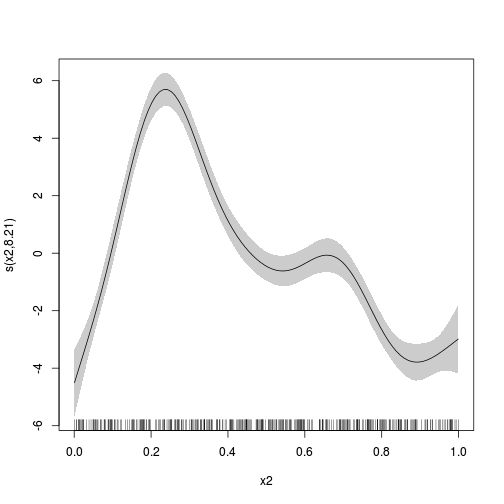
plot(dat.gam, pages = 1, scheme = 2)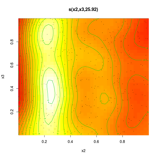
vis.gam(dat.gam, theta = 35)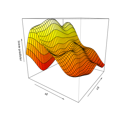
vis.gam(dat.gam, theta = 35, se = 2)